3.1 Explore data: main operations

STA141A: Fundamentals of Statistical Data Science

Akira Horiguchi

Quick note

Wickham and Grolemund (2017)

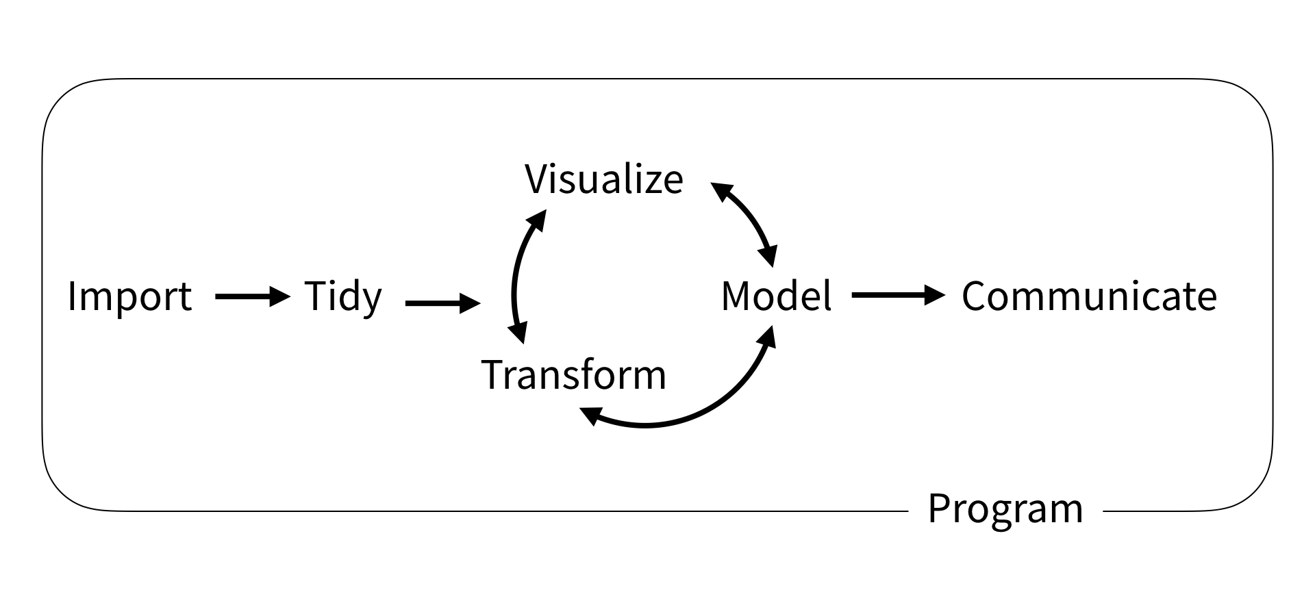
This next set of slides (3-4 lectures) is meant to get you started working with data: Import, Tidy, Transform, Visualize. (Modeling will be middle half of this course.)

By no means is it exhaustive.
Too much? Too little? Strongly depends on previous experience.
PRACTICE with basic tools to get comfortable before learning new ones.

`tidyverse`

`tidyverse` approach to data manipulation

Why use tidyverse over base R or data.table or other packages?

The tidyverse is an opinionated collection of R packages designed for data science. All packages share an underlying design philosophy, grammar, and data structures. — https://www.tidyverse.org/

Consistent syntax.
Many people work full-time (and get paid!) to make new packages, add new functionality, etc.
- In contrast, many other packages are created/maintained/updated by researchers who work on this part-time.

This slide deck will primarily use tidyverse solutions.

Reminder about packages

Packages are things we load using library().
If you haven’t installed a package PACKAGENAME before, you’ll get an error.
To install a package: install.packages("PACKAGENAME").
To load a package: library(PACKAGENAME).
For example:

install.packages("tidyverse")  # Do just once

library(tidyverse)  # Do at the start of every session

Load example dataset

library(nycflights13) # loads the `flights` tibble into environment
flights

# A tibble: 336,776 × 19
    year month   day dep_time sched_dep_time dep_delay arr_time sched_arr_time
   <int> <int> <int>    <int>          <int>     <dbl>    <int>          <int>
 1  2013     1     1      517            515         2      830            819
 2  2013     1     1      533            529         4      850            830
 3  2013     1     1      542            540         2      923            850
 4  2013     1     1      544            545        -1     1004           1022
 5  2013     1     1      554            600        -6      812            837
 6  2013     1     1      554            558        -4      740            728
 7  2013     1     1      555            600        -5      913            854
 8  2013     1     1      557            600        -3      709            723
 9  2013     1     1      557            600        -3      838            846
10  2013     1     1      558            600        -2      753            745
# ℹ 336,766 more rows
# ℹ 11 more variables: arr_delay <dbl>, carrier <chr>, flight <int>,
#   tailnum <chr>, origin <chr>, dest <chr>, air_time <dbl>, distance <dbl>,
#   hour <dbl>, minute <dbl>, time_hour <dttm>

Piping

The pipe operator |> allows you to write operations sequentially.

mean(flights$distance)

[1] 1039.913

Can instead pipe an output into the first argument of another function.

flights$distance |> mean()

[1] 1039.913

Can also use _ to specify which argument to pipe output to:

0.3 |> mean(flights$distance, trim=_)

[1] 869.0867

Piping

Can also use %>% (requires the magrittr package), which was used before R 4.1.0

You might see code using %>% or |>, depending on when the code was written/updated

Piping

Why pipe? Can be easier to read and understand.

# executed from "inside out"
mean(sqrt(log(flights$distance)))

[1] 2.580285

# executed from "left to right"
flights$distance |>
  log() |>
  sqrt() |>
  mean()

[1] 2.580285

Functions in tidyverse were designed with “first argument” piping in mind

Base R was created ~10 years before first pipe operator was introduced.
We will see more complex examples of this shortly.

Importing data

Introduction

We have seen data sets that are either built into base R or come from external packages

We will eventually want to import data from external files

Types of data files

CSV: comma separated values (this course will use this type the most)
TSV: tab separated values
FWF: fixed width file

To load files, the readr package has the following functions:

read_csv(), read_tsv(), read_delim()
read_fwf(), read_table()

`read_csv()`: can you spot the differences?

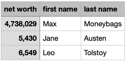
networth.csv

read.csv("networth.csv")  # from utils package; preinstalled with R

  net.worth first.name last.name
1 4,738,029        Max Moneybags
2     5,430       Jane    Austen
3     6,549        Leo   Tolstoy

read_csv("networth.csv")  # from readr package

# A tibble: 3 × 3
  `net worth` `first name` `last name`
        <dbl> <chr>        <chr>      
1     4738029 Max          Moneybags  
2        5430 Jane         Austen     
3        6549 Leo          Tolstoy

`read_csv()`: can you spot the differences?

Column names can have spaces. How to access?

nw_df <- read_csv("networth.csv")
nw_df

# A tibble: 3 × 3
  `net worth` `first name` `last name`
        <dbl> <chr>        <chr>      
1     4738029 Max          Moneybags  
2        5430 Jane         Austen     
3        6549 Leo          Tolstoy

nw_df$`net worth` * 10

[1] 47380290    54300    65490

You’ll likely want to use external files for your final project

For lecture, mostly stick with datasets from base R or packages

Subsetting a data frame

Subset based on data values (rather than row/column indices)

Column: select()
Row: filter()

The `select()` function

Returns a tibble with the columns specified, in order specified.

flights |>
  select(origin, dest, air_time, distance) |>  # Do not need quotation marks.
  colnames()

[1] "origin"   "dest"     "air_time" "distance"

flights |>
  select(distance, dest, origin, air_time) |>  # Do not need quotation marks.
  colnames()

[1] "distance" "dest"     "origin"   "air_time"

colnames(select(flights, distance, dest, origin, air_time))  # hard to read

[1] "distance" "dest"     "origin"   "air_time"

Helper functions for `select()`

starts_with("abc"): matches names that begin with “abc”.
ends_with("xyz"): matches names that end with “xyz”.
contains("ijk"): matches names that contain “ijk”.

flights |> colnames()

 [1] "year"           "month"          "day"            "dep_time"      
 [5] "sched_dep_time" "dep_delay"      "arr_time"       "sched_arr_time"
 [9] "arr_delay"      "carrier"        "flight"         "tailnum"       
[13] "origin"         "dest"           "air_time"       "distance"      
[17] "hour"           "minute"         "time_hour"

flights |> select(origin, dest, contains("sched"))

# A tibble: 336,776 × 4
   origin dest  sched_dep_time sched_arr_time
   <chr>  <chr>          <int>          <int>
 1 EWR    IAH              515            819
 2 LGA    IAH              529            830
...

The `filter()` function

# data = data to filter
# expr<#> = expression used to filter data, typically using ==, >, etc
filter(<data>, <expr1>)
filter(<data>, <expr1>, <expr2>, <expr3>)

Example: flights on February 15

filter(flights, month == 2, day == 15)

# A tibble: 954 × 19
    year month   day dep_time sched_dep_time dep_delay arr_time sched_arr_time
   <int> <int> <int>    <int>          <int>     <dbl>    <int>          <int>
 1  2013     2    15        3           2358         5      503            438
 2  2013     2    15        6           2115       171       48           2214
 3  2013     2    15        6           2250        76      117              5
 4  2013     2    15       22           2230       112      510            312
 5  2013     2    15       36           2352        44      607            437
...

flights |> filter(month == 2, day == 15)  # same as above

The `filter()` function

# data = data to filter
# expr = expression used to filter data, typically using ==, >, etc
filter(<data>, <expr>)

Expressions can be built up using comparison operators and logical operators.

& is “and”
| is “or”
! is “not”
%in% is a membership checker (is an object inside of a vector)
>, < mean greater than, less than
>=, <= mean greater than or equal to, less than or requal to
== means “is equal”
!= means “is not equal”

Examples of `filter()`

flights |>
  select(time_hour, origin, dest, air_time, distance) |>
  filter(distance < 120)

# A tibble: 2,076 × 5
   time_hour           origin dest  air_time distance
   <dttm>              <chr>  <chr>    <dbl>    <dbl>
 1 2013-01-01 09:00:00 LGA    PHL         32       96
 2 2013-01-01 13:00:00 EWR    BDL         25      116
 3 2013-01-01 16:00:00 JFK    PHL         35       94
...

flights |>
  select(time_hour, origin, dest, air_time, distance) |>
  filter(distance < 120, origin == 'EWR')

# A tibble: 493 × 5
   time_hour           origin dest  air_time distance
   <dttm>              <chr>  <chr>    <dbl>    <dbl>
 1 2013-01-01 13:00:00 EWR    BDL         25      116
 2 2013-01-01 22:00:00 EWR    BDL         24      116
...

Spot the error?

flights |>
  select(origin, dest, air_time, distance) |>
  filter(origin == SFO)

Spot the error?

flights |>
  select(origin, dest, air_time, distance) |>
  filter(origin == 'SFO')

Equivalent ways to filter on multiple conditions

flights |>
  select(origin, dest, air_time, distance) |>
  filter(distance < 120, origin == "EWR")

# A tibble: 493 × 4
   origin dest  air_time distance
   <chr>  <chr>    <dbl>    <dbl>
 1 EWR    BDL         25      116
 2 EWR    BDL         24      116
 3 EWR    BDL         24      116
...

flights |>
  select(origin, dest, air_time, distance) |>
  filter(distance < 120 & origin == "EWR")

flights |>
  select(origin, dest, air_time, distance) |>
  filter(distance < 120) |>
  filter(origin == "EWR")

Summarize a data frame

`count()`

To count occurrences of each unique value in a column:

dataframe |>
  count(column1, ...)

e.g., count \(\#\) of flights by origin:

flights |>
  count(origin)

# A tibble: 3 × 2
  origin      n
  <chr>   <int>
1 EWR    120835
2 JFK    111279
3 LGA    104662

Can also count occurrences for multiple columns:

flights |>
  count(origin, dest)

# A tibble: 224 × 3
   origin dest      n
   <chr>  <chr> <int>
 1 EWR    ALB     439
 2 EWR    ANC       8
 3 EWR    ATL    5022
 4 EWR    AUS     968
 5 EWR    AVL     265
 6 EWR    BDL     443
 7 EWR    BNA    2336
 8 EWR    BOS    5327
 9 EWR    BQN     297
10 EWR    BTV     931
# ℹ 214 more rows

`count()`

To count occurrences of each unique value in a column:

dataframe |>
  count(column1, ...)

e.g., want to count how many flights by origin:

flights |>
  count(origin)

# A tibble: 3 × 2
  origin      n
  <chr>   <int>
1 EWR    120835
2 JFK    111279
3 LGA    104662

Can also count occurrences for multiple columns:

flights |>
  count(origin, dest, sort=TRUE)

# A tibble: 224 × 3
   origin dest      n
   <chr>  <chr> <int>
 1 JFK    LAX   11262
 2 LGA    ATL   10263
 3 LGA    ORD    8857
 4 JFK    SFO    8204
 5 LGA    CLT    6168
 6 EWR    ORD    6100
 7 JFK    BOS    5898
 8 LGA    MIA    5781
 9 JFK    MCO    5464
10 EWR    BOS    5327
# ℹ 214 more rows

Summary statistics and missing data

Common summary statistics of interest in data:

Mean (mean())
Min/max (min(), max())
Median (median())
Standard deviation / variance (sd(), var())

R denotes missing data using NA. Typically, if you compute a function of a vector with NAs, it will return NA, unless you put na.rm=TRUE.

x <- c(-1, 0, 1, NA)
mean(x)

[1] NA

mean(x, na.rm=TRUE)

[1] 0

`summarise()`

If you want to compute summary statistics of dataframe, use summarise().

# data = data you want to create a new variable from
# new var name = the name your new variable will be
# calc exp = the calculation you want to perform
summarise(<data>, <new var name> = <calc exp>)

flights |>
  summarise(avg_dist = mean(distance))

# A tibble: 1 × 1
  avg_dist
     <dbl>
1    1040.

Computes summary for the entire dataset

`summarize()`

If you want to compute summary statistics of dataframe, use summarize().

# data = data you want to create a new variable from
# new var name = the name your new variable will be
# calc exp = the calculation you want to perform
summarize(<data>, <new var name> = <calc exp>)

flights |>
  summarize(avg_dist = mean(distance))

# A tibble: 1 × 1
  avg_dist
     <dbl>
1    1040.

Computes summary for the entire dataset

`group_by()` and `summarise()`

To compute summary statistics per category, use group_by() first.

flights |>
  summarize(median_distance = median(distance, na.rm=TRUE),
            max_air_time = max(air_time, na.rm=TRUE))

# A tibble: 1 × 2
  median_distance max_air_time
            <dbl>        <dbl>
1             872          695

flights |>
  group_by(origin) |>
  summarize(median_distance = median(distance, na.rm=TRUE),
            max_air_time = max(air_time, na.rm=TRUE))

# A tibble: 3 × 3
  origin median_distance max_air_time
  <chr>            <dbl>        <dbl>
1 EWR                872          695
2 JFK               1069          691
3 LGA                762          331

`group_by()` and `summarise()`

To compute summary statistics per category, use group_by() first.

flights |>
  summarize(median_distance = median(distance, na.rm=TRUE),
            max_air_time = max(air_time, na.rm=TRUE))

# A tibble: 1 × 2
  median_distance max_air_time
            <dbl>        <dbl>
1             872          695

flights |>
  group_by(origin, dest) |>  # can group by multiple variables
  summarize(median_distance = median(distance, na.rm=TRUE),
            max_air_time = max(air_time, na.rm=TRUE))

# A tibble: 224 × 4
# Groups:   origin [3]
   origin dest  median_distance max_air_time
   <chr>  <chr>           <dbl>        <dbl>
 1 EWR    ALB               143           50
 2 EWR    ANC              3370          434
 3 EWR    ATL               746          176
 4 EWR    AUS              1504          301
 5 EWR    AVL               583          119
 6 EWR    BDL               116           56
 7 EWR    BNA               748          176
 8 EWR    BOS               200          112
 9 EWR    BQN              1585          231
10 EWR    BTV               266           69
# ℹ 214 more rows

`mutate()`

adds new column(s) to the data frame using values from extant columns.

flights |>
  select(air_time, distance) |>
  mutate(hours = air_time / 60,
         mi_per_hour = distance / hours)

# A tibble: 336,776 × 4
   air_time distance hours mi_per_hour
      <dbl>    <dbl> <dbl>       <dbl>
 1      227     1400 3.78         370.
 2      227     1416 3.78         374.
 3      160     1089 2.67         408.
 4      183     1576 3.05         517.
 5      116      762 1.93         394.
 6      150      719 2.5          288.
...

mi_per_hour uses hours, which was created within the same mutate() call.

`mutate()`

adds new column(s) to the data frame using values from extant columns.

flights |>
  mutate(hours = air_time / 60,
         mi_per_hour = distance / hours, 
         .keep = "used")  # retains only the columns used in creating new columns

# A tibble: 336,776 × 4
   air_time distance hours mi_per_hour
      <dbl>    <dbl> <dbl>       <dbl>
 1      227     1400 3.78         370.
 2      227     1416 3.78         374.
 3      160     1089 2.67         408.
 4      183     1576 3.05         517.
 5      116      762 1.93         394.
 6      150      719 2.5          288.
...

mi_per_hour uses hours, which was created within the same mutate() call.

`mutate()`

adds new column(s) to the data frame using values from extant columns.

flights |>
  mutate(hours = air_time / 60,
         mi_per_hour = distance / hours, 
         .keep = "none")  # retains only grouping variables and the newly created columns

# A tibble: 336,776 × 2
   hours mi_per_hour
   <dbl>       <dbl>
 1 3.78         370.
 2 3.78         374.
 3 2.67         408.
 4 3.05         517.
 5 1.93         394.
 6 2.5          288.
...

mi_per_hour uses hours, which was created within the same mutate() call.

Complex calculations

Q: For each origin airport, compute the average flight time, in hours, for flights over 500 miles long.

colnames(flights)  # hint: use origin, air_time, distance

 [1] "year"           "month"          "day"            "dep_time"      
 [5] "sched_dep_time" "dep_delay"      "arr_time"       "sched_arr_time"
 [9] "arr_delay"      "carrier"        "flight"         "tailnum"       
[13] "origin"         "dest"           "air_time"       "distance"      
[17] "hour"           "minute"         "time_hour"

Complex calculations

Q: For each origin airport, compute the average flight time, in hours, for flights over 500 miles long.

flights |>
  mutate(air_time_hrs = air_time / 60) |>
  filter(distance > 500) |>
  group_by(origin) |>
  summarize(avg_flight_time_hrs = mean(air_time_hrs, na.rm=TRUE))

# A tibble: 3 × 2
  origin avg_flight_time_hrs
  <chr>                <dbl>
1 EWR                   2.99
2 JFK                   3.76
3 LGA                   2.27

Complex calculations

Q: For each origin airport, compute the average flight time, in hours, for flights over 500 miles long vs. less than or equal to 500 miles long.

colnames(flights)  # hint: use origin, air_time, distance

 [1] "year"           "month"          "day"            "dep_time"      
 [5] "sched_dep_time" "dep_delay"      "arr_time"       "sched_arr_time"
 [9] "arr_delay"      "carrier"        "flight"         "tailnum"       
[13] "origin"         "dest"           "air_time"       "distance"      
[17] "hour"           "minute"         "time_hour"

Complex calculations

Q: For each origin airport, compute the average flight time, in hours, for flights over 500 miles long vs. less than or equal to 500 miles long.

We will need to group_by() two variables:

origin airport
whether flight is \(> 500\) or \(\leq 500\) miles. (We need to create this variable.)

flights |>
  select(origin, air_time, distance) |>  # for visual clarity, not actually needed
  mutate(air_time_hrs = air_time / 60,
         distance_greater_500mi = distance > 500)

# A tibble: 336,776 × 5
   origin air_time distance air_time_hrs distance_greater_500mi
   <chr>     <dbl>    <dbl>        <dbl> <lgl>                 
 1 EWR         227     1400        3.78  TRUE                  
 2 LGA         227     1416        3.78  TRUE                  
 3 JFK         160     1089        2.67  TRUE                  
 4 JFK         183     1576        3.05  TRUE                  
...

Complex calculations

Q: For each origin airport, compute the average flight time, in hours, for flights over 500 miles long vs. less than or equal to 500 miles long.

flights |>
  mutate(air_time_hrs = air_time / 60,
         distance_greater_500mi = distance > 500) |>
  group_by(origin, distance_greater_500mi) |>
  summarize(avg_flight_time_hrs = mean(air_time_hrs, na.rm=TRUE))

# A tibble: 6 × 3
# Groups:   origin [3]
  origin distance_greater_500mi avg_flight_time_hrs
  <chr>  <lgl>                                <dbl>
1 EWR    FALSE                                0.900
2 EWR    TRUE                                 2.99 
3 JFK    FALSE                                0.849
4 JFK    TRUE                                 3.76 
5 LGA    FALSE                                0.916
6 LGA    TRUE                                 2.27

Reshaping a data frame

Tidy data

Multiple equivalent ways of organizing data into a dataframe.

table1
#> # A tibble: 6 × 4
#>   country      year  cases population
#>   <chr>       <dbl>  <dbl>      <dbl>
#> 1 Afghanistan  1999    745   19987071
#> 2 Afghanistan  2000   2666   20595360
#> 3 Brazil       1999  37737  172006362
#> 4 Brazil       2000  80488  174504898
#> 5 China        1999 212258 1272915272
#> 6 China        2000 213766 1280428583

table2
#> # A tibble: 12 × 4
#>   country      year type           count
#>   <chr>       <dbl> <chr>          <dbl>
#> 1 Afghanistan  1999 cases            745
#> 2 Afghanistan  1999 population  19987071
#> 3 Afghanistan  2000 cases           2666
#> 4 Afghanistan  2000 population  20595360
#> 5 Brazil       1999 cases          37737
#> 6 Brazil       1999 population 172006362
#> # ℹ 6 more rows

table1 is tidy - easier to work with using tidyverse.

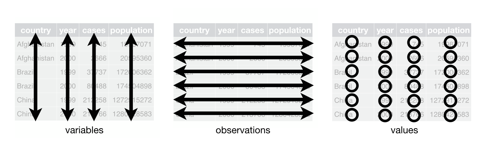
Tidy data

Each variable is a column; each column is a variable.
Each observation is a row; each row is an observation.
Each value is a cell; each cell is a single value.

Tidy data

Why tidy data?

Consistency - uniform format makes collaboration easier
Vectorization - R commands often operate on vectors of data, best for each column to be a vector of data

Tidying data

Unfortunately, most real-world datasets you encounter are NOT tidy.

A large part of “data scientist work” consists in tidying data (“cleaning data”).

billboard

# A tibble: 317 × 79
   artist     track date.entered   wk1   wk2   wk3   wk4   wk5   wk6   wk7   wk8
   <chr>      <chr> <date>       <dbl> <dbl> <dbl> <dbl> <dbl> <dbl> <dbl> <dbl>
 1 2 Pac      Baby… 2000-02-26      87    82    72    77    87    94    99    NA
 2 2Ge+her    The … 2000-09-02      91    87    92    NA    NA    NA    NA    NA
 3 3 Doors D… Kryp… 2000-04-08      81    70    68    67    66    57    54    53
 4 3 Doors D… Loser 2000-10-21      76    76    72    69    67    65    55    59
 5 504 Boyz   Wobb… 2000-04-15      57    34    25    17    17    31    36    49
 6 98^0       Give… 2000-08-19      51    39    34    26    26    19     2     2
 7 A*Teens    Danc… 2000-07-08      97    97    96    95   100    NA    NA    NA
...

Lengthening data with `pivot_longer()`

billboard

# A tibble: 317 × 79
   artist     track date.entered   wk1   wk2   wk3   wk4   wk5   wk6   wk7   wk8
   <chr>      <chr> <date>       <dbl> <dbl> <dbl> <dbl> <dbl> <dbl> <dbl> <dbl>
 1 2 Pac      Baby… 2000-02-26      87    82    72    77    87    94    99    NA
 2 2Ge+her    The … 2000-09-02      91    87    92    NA    NA    NA    NA    NA
 3 3 Doors D… Kryp… 2000-04-08      81    70    68    67    66    57    54    53
...

Each observation is a song.
First three columns (artist, track, date.entered) describe the song.
The next 76 columns (wk1, wk2, …, wk76) say song’s rank in each week.

If we want each observation to be a week ranking…

Each observation should be artist - track - date.entered - week - rank.
Each observation should be a row. Need to lengthen the dataframe.

Lengthening data with `pivot_longer()`

billboard |>
  pivot_longer(
    cols = starts_with("wk"),  # `cols`: which columns need to be pivoted
    names_to = "week",  # `names_to`: name of the column that the pivoted column names go
    values_to = "rank"  # `values_to`: name of the column that the pivoted cell values go
  )

# A tibble: 24,092 × 5
   artist track                   date.entered week   rank
   <chr>  <chr>                   <date>       <chr> <dbl>
 1 2 Pac  Baby Don't Cry (Keep... 2000-02-26   wk1      87
 2 2 Pac  Baby Don't Cry (Keep... 2000-02-26   wk2      82
 3 2 Pac  Baby Don't Cry (Keep... 2000-02-26   wk3      72
 4 2 Pac  Baby Don't Cry (Keep... 2000-02-26   wk4      77
...

“week” and “rank” do not appear as column names in billboard, so need quotes

Lengthening data with `pivot_longer()`

billboard |>
  pivot_longer(
    cols = starts_with("wk"),  # `cols`: which columns need to be pivoted
    names_to = "week",  # `names_to`: name of the column that the pivoted column names go
    values_to = "rank"  # `values_to`: name of the column that the pivoted cell values go
  )

# A tibble: 24,092 × 5
   artist track                   date.entered week   rank
   <chr>  <chr>                   <date>       <chr> <dbl>
 1 2 Pac  Baby Don't Cry (Keep... 2000-02-26   wk1      87
 2 2 Pac  Baby Don't Cry (Keep... 2000-02-26   wk2      82
 3 2 Pac  Baby Don't Cry (Keep... 2000-02-26   wk3      72
 4 2 Pac  Baby Don't Cry (Keep... 2000-02-26   wk4      77
...

Data is now tidy, but not ideal for data analysis. Why?

week should ideally be a number, not a character
Can use readr::parse_number() that extracts first number from string to fix.

Lengthening data with `pivot_longer()`

billboard |>
  pivot_longer(
    cols = starts_with("wk"),
    names_to = "week",
    values_to = "rank"
  ) |>
  mutate(week = parse_number(week))

# A tibble: 24,092 × 5
   artist track                   date.entered  week  rank
   <chr>  <chr>                   <date>       <dbl> <dbl>
 1 2 Pac  Baby Don't Cry (Keep... 2000-02-26       1    87
 2 2 Pac  Baby Don't Cry (Keep... 2000-02-26       2    82
 3 2 Pac  Baby Don't Cry (Keep... 2000-02-26       3    72
 4 2 Pac  Baby Don't Cry (Keep... 2000-02-26       4    77
...

Understanding `pivot_longer()`

Consider toy dataset: three people (A, B, C) each with two blood pressure (BP) measurements.

df <- tribble(
  ~id,  ~bp1, ~bp2,
   "A",  100,  120,
   "B",  140,  115,
   "C",  120,  125
)
df

# A tibble: 3 × 3
  id      bp1   bp2
  <chr> <dbl> <dbl>
1 A       100   120
2 B       140   115
3 C       120   125

Want each observation (id, bp) to have its own row:

df |>
  pivot_longer(
    cols = c(bp1, bp2),
    names_to = "measurement",
    values_to = "value"
  )

# A tibble: 6 × 3
  id    measurement value
  <chr> <chr>       <dbl>
1 A     bp1           100
2 A     bp2           120
3 B     bp1           140
4 B     bp2           115
5 C     bp1           120
6 C     bp2           125

Understanding `pivot_longer()`

df |>
  pivot_longer(
    cols = c(bp1, bp2),  # which columns need to be pivoted
    names_to = "measurement",  # name of the column that the pivoted column names go
    values_to = "value"  # name of the column that the pivoted cell values go
  )

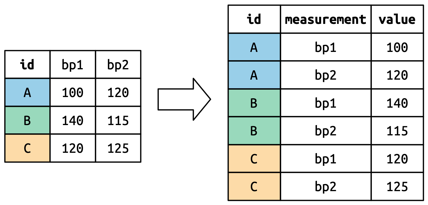
Values in columns that are already variables (here, id) need to be repeated for each pivoted column.

Understanding `pivot_longer()`

df |>
  pivot_longer(
    cols = c(bp1, bp2),  # which columns need to be pivoted
    names_to = "measurement",  # name of the column that the pivoted column names go
    values_to = "value"  # name of the column that the pivoted cell values go
  )

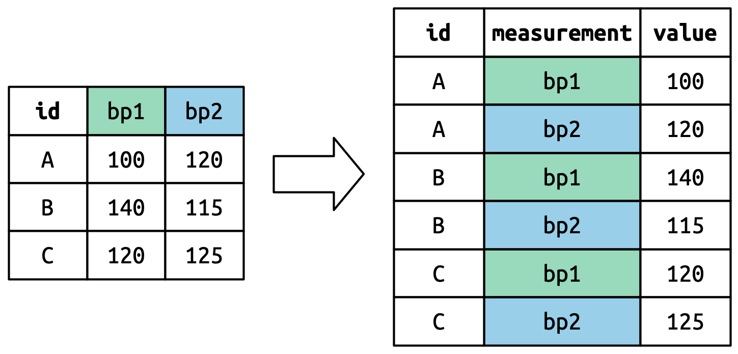
Pivoted column names bp1,bp2 become values in new column "measurement"; values repeated for each row in df.

Understanding `pivot_longer()`

df |>
  pivot_longer(
    cols = c(bp1, bp2),  # which columns need to be pivoted
    names_to = "measurement",  # name of the column that the pivoted column names go
    values_to = "value"  # name of the column that the pivoted cell values go
  )

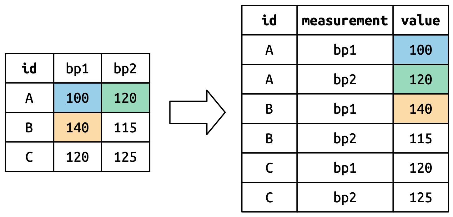
Cell values are values in a new variable, with name values_to, unwound row by row.

Widening data

We’ll now use pivot_wider() to widen data which is (too) long.

cms_patient_experience <- tidyr::cms_patient_experience |> 
   select(-measure_title)
cms_patient_experience

# A tibble: 500 × 4
   org_pac_id org_nm                               measure_cd   prf_rate
   <chr>      <chr>                                <chr>           <dbl>
 1 0446157747 USC CARE MEDICAL GROUP INC           CAHPS_GRP_1        63
 2 0446157747 USC CARE MEDICAL GROUP INC           CAHPS_GRP_2        87
 3 0446157747 USC CARE MEDICAL GROUP INC           CAHPS_GRP_3        86
 4 0446157747 USC CARE MEDICAL GROUP INC           CAHPS_GRP_5        57
 5 0446157747 USC CARE MEDICAL GROUP INC           CAHPS_GRP_8        85
 6 0446157747 USC CARE MEDICAL GROUP INC           CAHPS_GRP_12       24
 7 0446162697 ASSOCIATION OF UNIVERSITY PHYSICIANS CAHPS_GRP_1        59
...

The basic unit studied is an organization, but it’s spread across six rows for different measurements.

Widening data

cms_patient_experience |>
  pivot_wider(
    id_cols = starts_with("org"), # org_pac_id and org_nm are identifiers
    names_from = measure_cd,
    values_from = prf_rate
  )

# A tibble: 95 × 8
   org_pac_id org_nm CAHPS_GRP_1 CAHPS_GRP_2 CAHPS_GRP_3 CAHPS_GRP_5 CAHPS_GRP_8
   <chr>      <chr>        <dbl>       <dbl>       <dbl>       <dbl>       <dbl>
 1 0446157747 USC C…          63          87          86          57          85
 2 0446162697 ASSOC…          59          85          83          63          88
 3 0547164295 BEAVE…          49          NA          75          44          73
 4 0749333730 CAPE …          67          84          85          65          82
 5 0840104360 ALLIA…          66          87          87          64          87
 6 0840109864 REX H…          73          87          84          67          91
...

If you don’t supply id_cols, R assumes that all columns EXCEPT for names_from and values_from are id_cols.

Understanding `pivot_wider()`

Dataset where two patients (A, B), with between 2 and 3 BP measurements.

df

# A tibble: 5 × 3
  id    measurement value
  <chr> <chr>       <dbl>
1 A     bp1           100
2 B     bp1           140
3 B     bp2           115
4 A     bp2           120
5 A     bp3           105

df |>
  pivot_wider(
    names_from = measurement,
    values_from = value
  )

# A tibble: 2 × 4
  id      bp1   bp2   bp3
  <chr> <dbl> <dbl> <dbl>
1 A       100   120   105
2 B       140   115    NA

There is no measurement for bp3 for B, so R puts in NA.
id_cols is empty, so R assumes that all columns EXCEPT for names_from and values_from are id_cols.

Going from long to wide and back again

df

# A tibble: 5 × 3
  id    measurement value
  <chr> <chr>       <dbl>
1 A     bp1           100
2 B     bp1           140
3 B     bp2           115
4 A     bp2           120
5 A     bp3           105

(wide_df <- df |>
  pivot_wider(
    names_from = measurement,
    values_from = value
  ) )

# A tibble: 2 × 4
  id      bp1   bp2   bp3
  <chr> <dbl> <dbl> <dbl>
1 A       100   120   105
2 B       140   115    NA

(long_df <- wide_df |>
    pivot_longer(
      cols = c(bp1, bp2, bp3),
      names_to = "measurement",
      values_to = "value"))

# A tibble: 6 × 3
  id    measurement value
  <chr> <chr>       <dbl>
1 A     bp1           100
2 A     bp2           120
3 A     bp3           105
4 B     bp1           140
5 B     bp2           115
6 B     bp3            NA

We now have an additional row to account for the NA.

Tidy check

df

# A tibble: 8 × 4
  City  Date       Measurement Value
  <chr> <chr>      <chr>       <dbl>
1 CityA 2024-01-01 Temperature    20
2 CityA 2024-01-01 Humidity       80
3 CityA 2024-01-02 Temperature    22
4 CityA 2024-01-02 Humidity       82
5 CityB 2024-01-01 Temperature    18
6 CityB 2024-01-01 Humidity       85
7 CityB 2024-01-02 Temperature    19
8 CityB 2024-01-02 Humidity       88

Not tidy, since each variable is not a column, e.g. temperature/humidity.
“Tidyness” can be a bit ambiguous, but if a column has different units (e.g., degrees vs. % humidity), likely not tidy.
Q: How do we make the table wider?

Tidy check

df |>
  pivot_wider(
    names_from = Measurement,
    values_from = Value
  )

# A tibble: 4 × 4
  City  Date       Temperature Humidity
  <chr> <chr>            <dbl>    <dbl>
1 CityA 2024-01-01          20       80
2 CityA 2024-01-02          22       82
3 CityB 2024-01-01          18       85
4 CityB 2024-01-02          19       88

Tidy check

scores

# A tibble: 3 × 3
  Student  Math  Chem
  <chr>   <dbl> <dbl>
1 Ant        85    90
2 Bug        92    78
3 Cat        88    95

Make scores longer by having a column called Subject with values "Math" and "Chem".

Q: Is the following code correct?

scores |>
  pivot_longer(
    cols = c(Math, Chem),
    names_to = Subject,
    values_to = Score
  )

No: scores tries to refer to Subject and Score which are not columns.

scores |>
  pivot_longer(
    cols = c(Math, Chem),
    names_to = "Subject",
    values_to = "Score"
  )

# A tibble: 6 × 3
  Student Subject Score
  <chr>   <chr>   <dbl>
1 Ant     Math       85
2 Ant     Chem       90
3 Bug     Math       92
4 Bug     Chem       78
5 Cat     Math       88
6 Cat     Chem       95

3.1 Explore data: main operations

Quick note

tidyverse

tidyverse approach to data manipulation

Reminder about packages

Load example dataset

Piping

Piping

Piping

Importing data

Introduction

read_csv(): can you spot the differences?

read_csv(): can you spot the differences?

Subsetting a data frame

Subset based on data values (rather than row/column indices)

The select() function

Helper functions for select()

The filter() function

The filter() function

Examples of filter()

Spot the error?

Spot the error?

Equivalent ways to filter on multiple conditions

Summarize a data frame

count()

count()

Summary statistics and missing data

summarise()

summarize()

group_by() and summarise()

group_by() and summarise()

mutate()

mutate()

mutate()

mutate()

Complex calculations

Complex calculations

Complex calculations

Complex calculations

Complex calculations

Reshaping a data frame

Tidy data

Tidy data

Tidying data

Lengthening data with pivot_longer()

Lengthening data with pivot_longer()

Lengthening data with pivot_longer()

Lengthening data with pivot_longer()

Understanding pivot_longer()

Understanding pivot_longer()

Understanding pivot_longer()

Understanding pivot_longer()

Widening data

Widening data

Understanding pivot_wider()

Going from long to wide and back again

Tidy check

Tidy check

Tidy check

`tidyverse`

`tidyverse` approach to data manipulation

`read_csv()`: can you spot the differences?

`read_csv()`: can you spot the differences?

The `select()` function

Helper functions for `select()`

The `filter()` function

The `filter()` function

Examples of `filter()`

`count()`

`count()`

`summarise()`

`summarize()`

`group_by()` and `summarise()`

`group_by()` and `summarise()`

`mutate()`

`mutate()`

`mutate()`

`mutate()`

Lengthening data with `pivot_longer()`

Lengthening data with `pivot_longer()`

Lengthening data with `pivot_longer()`

Lengthening data with `pivot_longer()`

Understanding `pivot_longer()`

Understanding `pivot_longer()`

Understanding `pivot_longer()`

Understanding `pivot_longer()`

Understanding `pivot_wider()`