Inference for comparing many means

STA35B: Statistical Data Science 2

Akira Horiguchi

Table of contents

• Many populations
• ANOVA
• Example: class exam
• Consider the following toy ANOVA Data
• F statistic
• F statistic
• Example: class exam
• Class Data Randomization Test
• Test statistic for three or more means is an F statistic
• Mathematical model, test for comparing 3+ means
• Examples: class exams
• ANOVA with lm and anova
• Example: Batting in MLB
• Reconstructing ANOVA Output

Based on Ch 22 of IMS

library(tidyverse)
library(openintro)
library(infer)

library(knitr)
library(ggpubr)
library(kableExtra)
library(gghighlight)

library(scales) # label_dollar

options(pillar.print_min = 9)  # to avoid annoying scroll behavior
knitr::opts_chunk$set(out.height = "100%")
theme_set(theme_bw() + theme(axis.text = element_text(size = 14), 
                             axis.title = element_text(size = 16), 
                             ))

Many populations

We saw previously how to compare population means of two populations.

• Suppose we want to compare means across many populations (e.g., SAT scores by city).
• Imagine doing all pairwise comparisons:
  • LA vs SF, SF vs San Jose, Davis vs San Jose, …
• However, as we do more and more comparisons, likely that we will see differences in data that are solely due to random chance.
  • We will discuss this for our final lecture.
• We will instead perform a single comparison incorporating all populations.
• This is the goal of the analysis of variance (ANOVA) technique which we will talk about today.

ANOVA

ANOVA uses a single hypothesis test to check whether means across many groups are equal. If \(k\) groups,

• \(H_0\): All \(k\) groups share the same mean outcome: \[\mu_1 = \mu_2 = \cdots = \mu_k\] where \(\mu_j\) represents the mean of the outcome for observations in group \(j.\)
• \(H_A\): At least one mean is different.

Must check three conditions on the data before performing ANOVA:

• the observations are independent within and between groups,
• the responses within each group are nearly normal, and
• the variability across the groups is about equal.

Example: class exam

Consider three sections of the same intro stats course.

• Are there substantial differences between these three sections (A, B, and C) in the first midterm exam scores?

Appropriate hypotheses may be written in the following form:

• \(H_0\): The average score is identical in all sections, \[\mu_A = \mu_B = \mu_C.\] Assuming each section is equally difficult, the observed difference in exam scores is due to chance.
• \(H_A\): The average score varies by class. We would reject the null hypothesis in favor of the alternative hypothesis if there were larger differences among the class averages than what we might expect from chance alone.

In ANOVA, strong evidence favoring the alternative hypothesis typically comes from unusually large differences in the group means.

• Key to assessing this: look at how much the means differ relative to the variability of individual observations within each group.

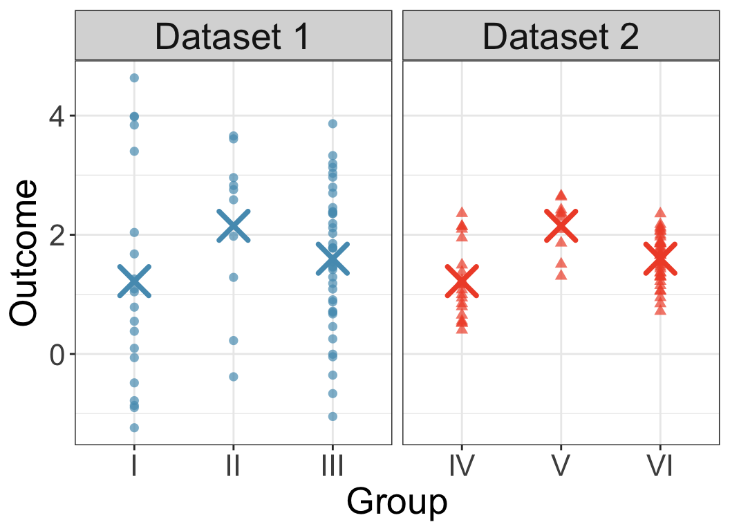
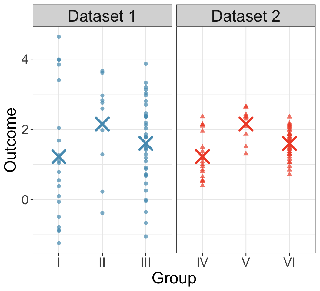
Consider the following toy ANOVA Data

Does it look like the diffrnces in group means could come from random chance?

• Compare I vs II vs III, then compare IV vs V vs VI
  • group I has same center as group IV;
    group II has same center as group V;
    group III has same center as group VI.

Figure 1: Data shown as points. Crosses indicate group means.

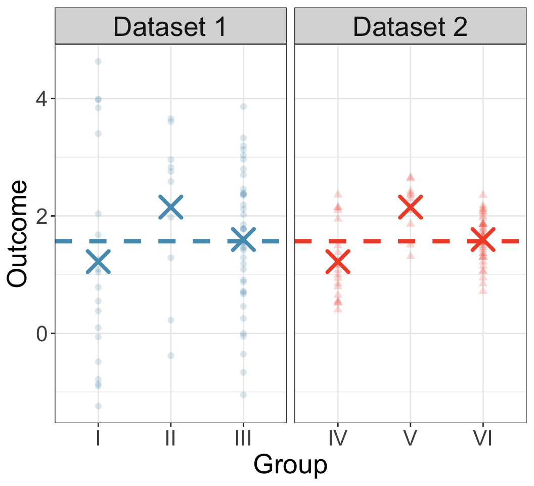
Consider the ratio \[\frac{\text{between-group variability}}{\text{within-group variability}}\]

• What does this look like for Groups I/II/III? For groups IV/V/VI?
• What does a large ratio value suggest?
  What does a small ratio value suggest?

(see next slide)

Groups I/II/III: it is plausible that difference in group centers is due to random chance.

Groups IV/V/VI: difference in group centers seem large relative to variability within each group, possibly due to true differences across groups.

F statistic

Goal: assess whether the observed variability in sample group means is due to random chance.

• For between-group variability, consider the sum of squares between groups (SSG): \[SSG = \sum_{j=1}^k n_j (\bar x_j - \bar x)^2\]
  • \(k\) is the number of means we are comparing;
  • \(n_j\) is the number of observations in group \(j\);
  • \(\bar x_j\) is the sample mean of group \(j\);
  • \(\bar x\) is the overall sample mean across all observations.
• For within-group variability, consider the sum of squares errors (SSE): \[\begin{align*}SSE&= \sum_{j=1}^k \sum_{i=1}^{n_j} ( x_{j,i} - \bar x_j)^2\end{align*}\]

SSG: variability of group means (weighted by group size)

SSE: variability within each group

Data shown as points. Crosses indicate group means.

F statistic

It turns out that the sum of squares total (SST) \[SST \;\;=\;\; \sum_{i=1}^n (x_i - \bar x)^2\] is the sum of SSG and SSE: \[SST \;\;=\;\; SSG + SSE\] which can be shown using a bunch of algebra.

(Note: I am using the textbook’s abbreviations for SSG, SSE, and SST. For this course, I would like you to do the same. But other texts may use different abbreviations, such as total sum of squares (TSS), and SST might refer to sum of squares for treatment, which is our SSG. Therefore, it is very important that you understand what each abbreviation means and the intuition behind them, and not just memorize the abbreviations.)

For reasons we’ll see later, we’ll want to use scaled versions of SSG and SSE:

• The mean square between groups (MSG) is a scaled version of SSG;
  the mean squared errors (MSE) is a scaled version of SSE:

\[\begin{align*} MSG &\;\;=\;\; \frac{1}{\mathsf{df}_G} SSG \;\;=\;\; \frac{1}{k-1} SSG,\newline MSE&\;\;=\;\;\frac{1}{\mathsf{df}_E} SSE \;\;=\;\;\frac{1}{n-k} SSE.\end{align*}\]

The F statistic is defined to be ratio of these two: \[F \;=\; \frac{MSG}{MSE}.\]

• Typically use software to compute. Not worth doing by hand.

Let’s now do a randomization test using this F statistic to see if the differences in means are likely due to random chance or not.

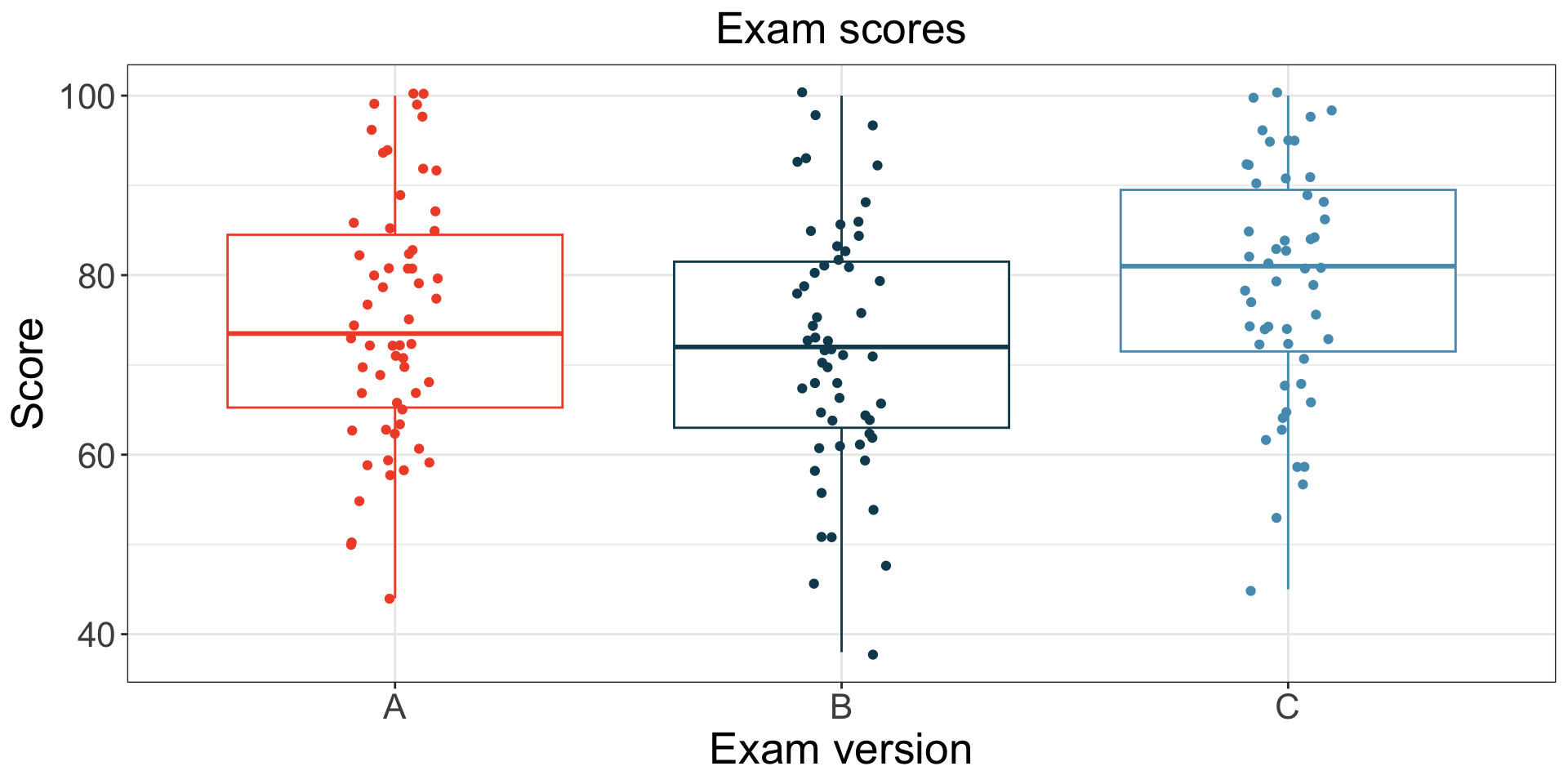
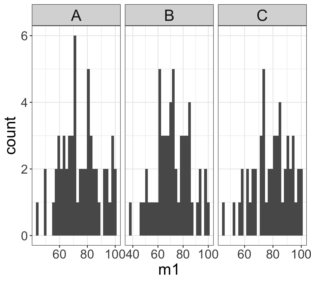
Example: class exam

A teacher gave three versions (A, B, C) of an exam.

• Data is summarized in table/plot to the right.
• Is the exam difficulty the same across the three versions?

Hypothesis test:

• \(H_0\): All three versions are equally difficult. \[\mu_A = \mu_B = \mu_C\]
• \(H_A\): At least one version is inherently more (or less) difficult than the others.

Version	n	Mean	SD	Min	Max
A	58	75.1	13.9	44	100
B	55	72.0	13.8	38	100
C	51	78.9	13.1	45	100

Figure 2: Exam scores for each of the three sections.

Class Data Randomization Test

Randomization test with many means: same idea as in two means.

• Null assumption: versions are equally difficult.
• Exam version (A or B or C) is randomly allocated to the exam scores, under the null assumption.

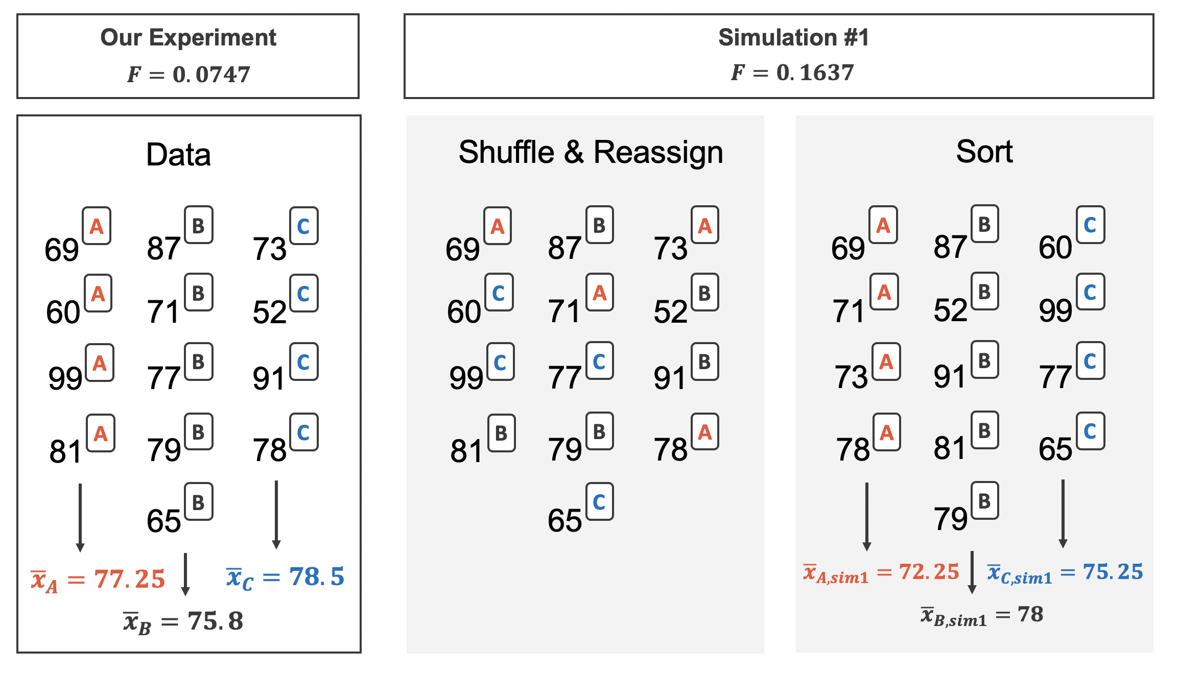
• For each simulation, we calculate the F statistic.

Figure 3: Histogram of 10,000 randomized F statistics.

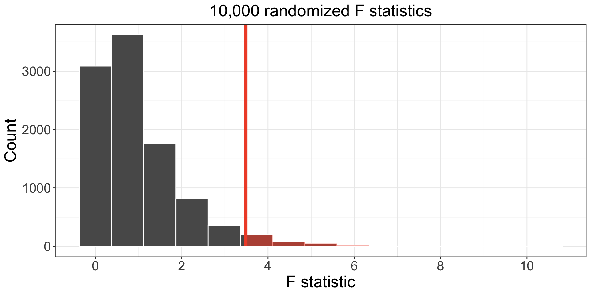
• 297 of 10,000 simulations had an F statistic greater than or equal to the observed value 3.48.
• p-value 0.0297 is below 0.05, so we reject \(H_0\).
• Conclusion: our observed value is unlikely due to chance if all exams were equally difficult.

Test statistic for three or more means is an F statistic

Recall: the F statistic is a ratio of how the groups differ (MSG) as compared to how the observations within a group vary (MSE).

\[F = \frac{MSG}{MSE}\]

• When the \(H_0\) is true and the conditions below are met, the F statistic follows an F distribution with parameters \(df_1 = k-1\) and \(df_2 = n-k.\)

Conditions:

• the observations are independent within and between groups,
• the responses within each group are nearly normal, and
• the variability across the groups is about equal.

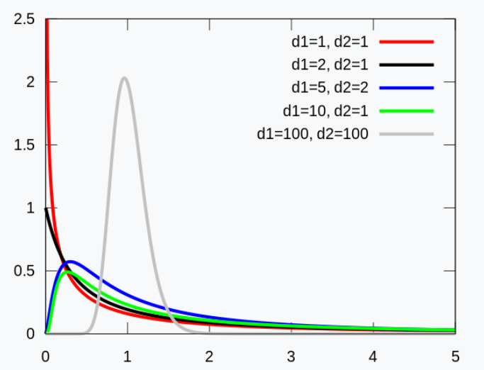
F distribution

• is determined by two parameters, \(df_1\) and \(df_2\), representing deg of freedom
• is always non-negative, so it does NOT look like t or normal distribution

Mathematical model, test for comparing 3+ means

The F-distribution allows us to use a mathematical approach to evaluate the null hypothesis.

• The \(p\)-value for the problem is given by the area under the F-distribution curve to the right of the observed F-statistic value.

  • Also known as the “right-tail area”

• Functions in R can be used to calculate percentiles and areas for F statistics

  • pnorm(), pt(), pf() - percent of data to the left of a certain value
  • qnorm(), qt(), qf() - value corresponding to data at a certain percentile

Examples: class exams

• So if we return to the data here

Version	n	Mean	SD	Min	Max
A	58	75.1	13.9	44	100
B	55	72.0	13.8	38	100
C	51	78.9	13.1	45	100

• The F statistic for this data was 3.48

• Mathematical approach for calculating \(p\)-value:

df1 <- 3 - 1  # k-1
df2 <- 58+55+51 - 3  # n-k
pf(3.48, df1 = df1, df2 = df2)

[1] 0.9668556

• Only 3.3% of data is to the right of 3.48
• \(p\)-value of 0.033 < 0.05 - can reject the null hypothesis

ANOVA with lm and anova

Alternatively, we can perform analysis of variance using lm() and anova():

(lm_class <- lm(m1 ~ exam, data = classdata))

Call:
lm(formula = m1 ~ exam, data = classdata)

Coefficients:
(Intercept)        examB        examC  
     75.103       -3.140        3.838  

anova(lm_class) |> broom::tidy() |> kable(digits=c(0, 0, 0, 0, 3, 3))

term	df	sumsq	meansq	statistic	p.value
exam	2	1290	645	3.484	0.033
Residuals	161	29810	185	NA	NA

• df: degrees of freedom \(df_1=k-1\) and \(df_2=n-k\)
• sumsq: SSG (top) and SSE (bottom)
• meansq: MSG (top) and MSE (bottom)
• statistic: F statistic: \(F = \frac{MSG}{MSE}\)
• p.value: p-value for the F statistic

Is this p-value valid? Need to check conditions:

• Independence: if data comes from simple random sample, this holds. For students we aren’t sure, so this might present problems, but let’s assume it’s OK
• Approximate normality - when sample size is large and no extreme outliers, then this is ok
• Approximately constant variance - each group has approximately the same variance

• Thus, we can use to reject \(H_0\) under 0.05 discernibiliity level.

Example: Batting in MLB

Does batting performance of baseball players differs according to position?

• Outfielder (OF)
• Infielder (OF)
• Catcher (C)

Data: 429 Major League Baseball (MLB) players from 2018, each \(\geq 100\) at bats.

• Does the on-base percentage (OBP) differ across these 3 groups?

• Some variables and descriptions:

# A tibble: 4 × 2
  variable col1                                       
  <chr>    <chr>                                      
1 name     Player name                                
2 team     abbreviated name of the player's team      
3 position player's primary field position (OF, IF, C)
4 OBP      On-base percentage                         

• First few rows:

name	team	position	OBP
Abreu, J	CWS	IF	0.325
Acuna Jr., R	ATL	OF	0.366
Adames, W	TB	IF	0.348
Adams, M	STL	IF	0.309

• position has three levels:

unique(mlb_players_18$position)

[1] OF IF C 
Levels: OF IF C

Null and alternative hypotheses:

• \(H_0\): the OBP for these three positions is the same; \[\mu_{OF} = \mu_{IF} = \mu_C\]
• \(H_A\): there is some difference among these three groups: \[\mu_{OF} \neq \mu_{IF}, \quad \mu_{IF} \neq \mu_C, \quad\text{or}\quad \mu_{OF} \neq \mu_C\]

ANOVA analysis

First, we need to check the conditions for F statistic / ANOVA analysis to hold.

• Independence: if data comes from simple random sample, this holds. For MLB we aren’t sure, so this might present problems, but let’s assume it’s OK
• Approximate normality - when sample size is large and no extreme outliers, then this is ok
• Approximately constant variance - variance within each group is approximately the same across groups

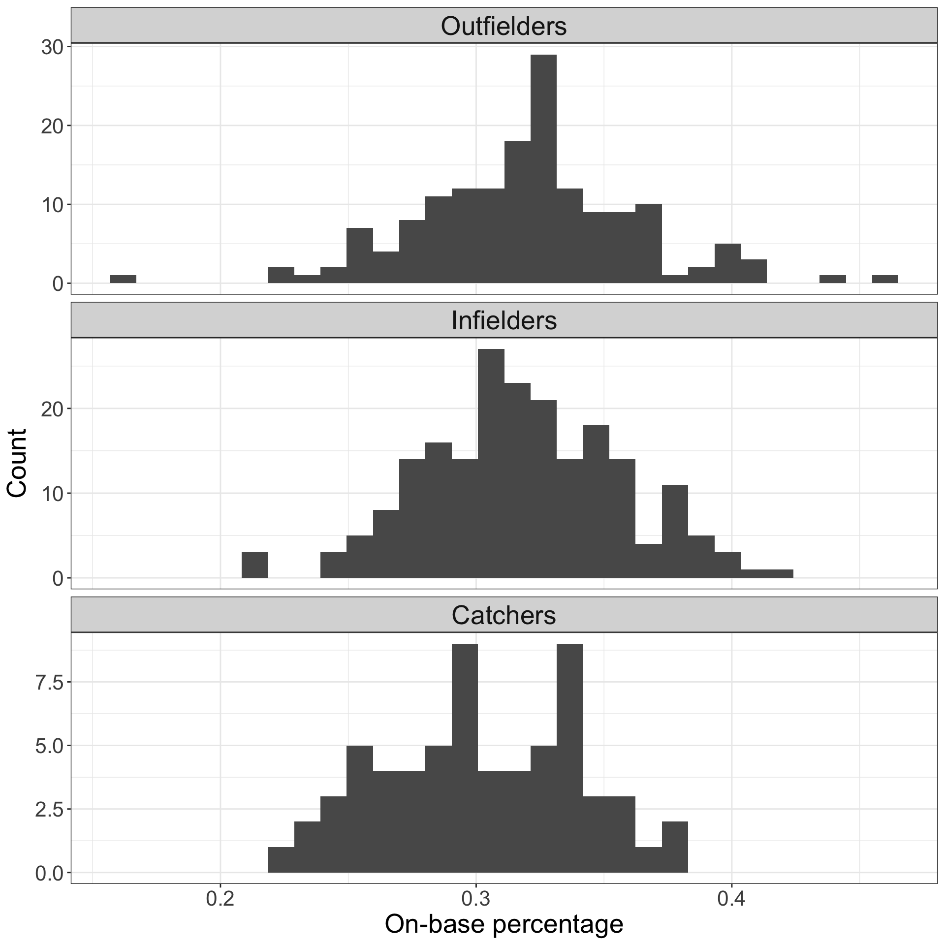
• Does appear to be approximately normal, no extreme outliers
• We see that variability across the groups is quite similar
• So our F statistic analysis can proceed

MLB ANOVA Output

To do analysis of variance, we use lm() and anova():

(mod <- lm(OBP~position, data=mlb_players_18))

Call:
lm(formula = OBP ~ position, data = mlb_players_18)

Coefficients:
(Intercept)   positionIF    positionC  
   0.319819    -0.001433    -0.017881  

anova(mod) |> 
    broom::tidy() |> 
    kable(digits=c(0,0,3,4,2,3))

term	df	sumsq	meansq	statistic	p.value
position	2	0.016	0.0080	5.08	0.007
Residuals	426	0.674	0.0016	NA	NA

How to read ANOVA output table?

• df: degrees of freedom \(df_1=k-1\) and \(df_2=n-k\)
• sumsq: SSG (top) and SSE (bottom)
• meansq: MSG (top) and MSE (bottom)
• statistic: F statistic: \(F = \frac{MSG}{MSE}\)
• p.value: p-value for the F statistic
  • p-value is smaller than 0.05, so we can reject the null hypothesis

Can derive this entire tibble by using just df and sumsq (and pf() to calc p-value from the statistic)

• meansq: sumsq divided by df
• statistic: quotient of the two meansq values
• For p.value, can use pf:

1 - pf(5.077, df1 = 2, df2 = 426)

[1] 0.006621471

Reconstructing ANOVA Output

Can derive this entire tibble by using just df and sumsq (and pf() to calc p-value from the statistic)

• meansq: sumsq divided by df
• statistic: quotient of the two meansq values
• For p.value, can use pf:

1 - pf(statistic, df1 = df1, df2 = df2)

Let’s try it

term	df	sumsq	meansq	statistic	p.value
position	2	0.016	X	X	X
Residuals	426	0.674	X	NA	NA