Inference for Comparing Paired Means

STA35B: Statistical Data Science 2

Akira Horiguchi

Table of contents

• The Big Idea
• Notation
• Comparison
• Randomization Test for Pairs
• Bootstrap CI for Paired Differences
• Mathematical Model
• Which Method Should We Use?

Based on Ch 21 of IMS

library(tidyverse)
library(openintro)
library(infer)

library(knitr)
library(ggpubr)
library(kableExtra)
library(gghighlight)

library(scales) # label_dollar

options(pillar.print_min = 9)  # to avoid annoying scroll behavior
knitr::opts_chunk$set(out.height = "100%")
theme_set(theme_bw() + theme(axis.text = element_text(size = 14), 
                             axis.title = element_text(size = 16), 
                             ))

The Big Idea

Timing: 2 minutes. Contrast with Chapter 20: independent groups require that knowing one observation does not tell us about another. In paired data, the dependence is the feature.

Two sets of observations are paired if each observation in one set has a special correspondence with exactly one observation in the other set. Examples:

Observational unit	Comparison groups	Measurement
Car	Smooth Turn vs. Quick Spin tire	tread remaining
Textbook	UCLA bookstore vs. Amazon	new-book price
Student	pre-course vs. post-course	exam score

Paired data represent a particular type of experimental structure where

• the analysis is somewhat akin to a one-sample analysis
• but has other features that resemble a two-sample analysis

Timing: 2 minutes. Ask students what the observational unit is in each row. The observational unit is the thing that creates the pair.

Why Pairing Helps

Pairing can reduce noise when paired observations are similar. Example:

• Some books are expensive everywhere.
• Some students start with higher baseline scores.
• Some cars wear tires faster than others.

By comparing within pairs, we remove much of that background variation.

Check: Paired or Not?

For each setting, decide whether a paired analysis is appropriate.

1. Pre-test and post-test scores for the same students.
2. Salaries from a random sample of men and a separate random sample of women.
3. Target and Walmart prices for the same 50 items.
4. SAT scores from 100 students at one high school and 100 students at another.

Timing: 2.5 minutes. Paired: 1 and 3. Not paired: 2 and 4. Ask students to identify the observational unit and the pairing link.

Notation

Typically the value of interest is the difference in measurements.

• Let \(x_{i,1}\) be the measurement of unit \(i\) under condition 1.
• Let \(x_{i,2}\) be the measurement of unit \(i\) under condition 2.

For each pair (\(x_{i,1}\), \(x_{i,2}\)), compute one difference:

\[ d_i = x_{i,1} - x_{i,2} \]

Then analyze:

\[ d_1, d_2, \ldots, d_n \]

as a single quantitative sample.

The parameter is the mean paired difference: \(\mu_d\).

Check: Small Calculation

Six students take a quiz before and after a short lesson.

Student	Before	After
1	6	8
2	7	8
3	5	6
4	8	9
5	6	7
6	7	9

Use \(d_i = After - Before\).

1. Compute the six differences.

Timing: 2 minutes. Emphasize consistent subtraction order. Switching the order changes the sign but not the evidence.

Comparison

If mathematical modeling is chosen as the analysis tool, paired data inference on the difference in measurements will be identical to the one-sample mathematical techniques (Ch 19).

• However, recall that with pure one-sample data, the computational tools for hypothesis testing are not easy to implement and were not presented.
• With paired data, the randomization test fits nicely with the structure of the experiment and is presented here.

Randomization Test for Pairs

Let’s examine this procedure in the context of the following study.

Tire Tread Study

Research question: After 1,000 miles of driving, do Smooth Turn and Quick Spin tires have different average tread remaining?

Design:

• 25 cars
• each car gets one tire of each brand
• tread is measured after 1,000 miles

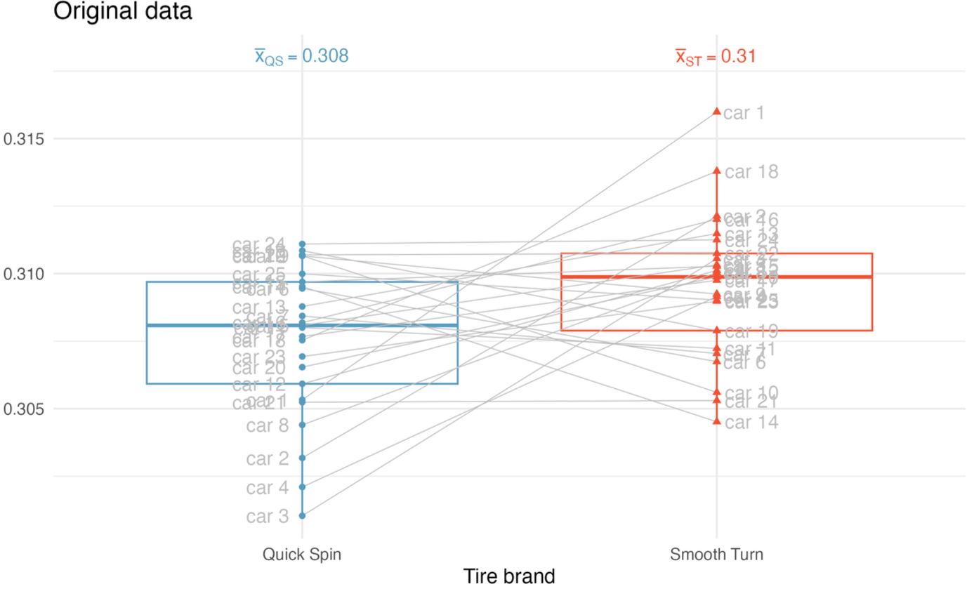
Figure 1: Observed tire data.

Observed means:

\[ \bar{x}_{Smooth} = 0.310,\quad \bar{x}_{Quick} = 0.308 \]

Timing: 2 minutes. The car is the pair. Road conditions, driving style, and potholes are shared within a car, so comparing tires within a car is valuable.

Define:

\[ d_i = \text{Smooth Turn tread}_i - \text{Quick Spin tread}_i \]

Then:

\[ \bar{d} = 0.310 - 0.308 = 0.002 \]

Hypotheses:

\[ H_0: \mu_d = 0 \qquad H_A: \mu_d \ne 0 \]

Timing: 2 minutes. A mean difference of 0.002 cm is small in raw units. The inferential question is whether that difference is large relative to natural within-car variability.

Randomization Test for Pairs

Under \(H_0\), tire brand should not matter within a car. So, for each car:

• keep the two tread measurements together (the pair structure stays intact!),
• randomly decide whether to keep or swap the brand labels,
• compute the mean paired difference,
• repeat many times.

Timing: 3 minutes. This is the paired-data version of randomization. We do not shuffle all tire measurements freely; we only swap labels within the car because the car creates the pair.

What Changes?

• Independent two-sample randomization: shuffle group labels across all observations.
• Paired randomization: swap labels within each pair.

Timing: 2 minutes. Draw two cars on the board. Each car keeps two tire measurements. The randomization only decides which value is labeled Smooth Turn and which is labeled Quick Spin.

Tire Study: Conclusion

Figure 2: Histogram of 1,000 mean differences with tire brand randomly assigned across the two tread measurements (in cm) per pair.

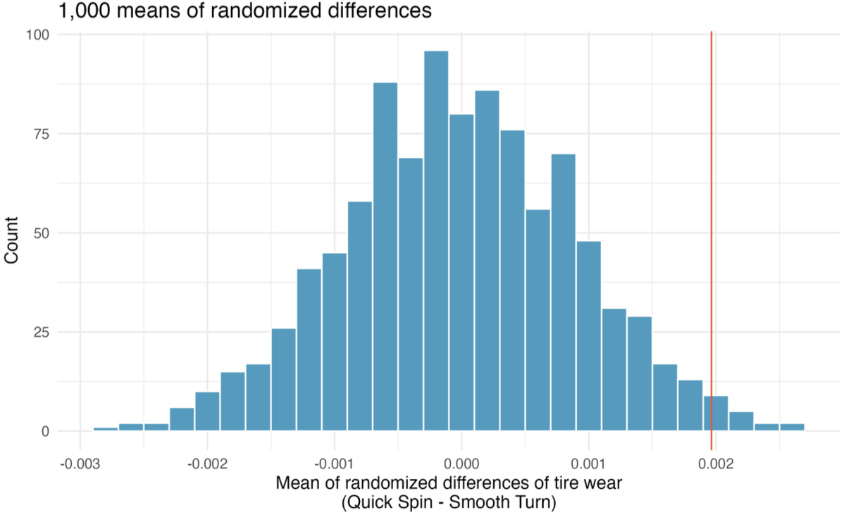
• Randomization distribution is centered near 0 because it is generated under \(H_0\).
• The observed mean difference, \(\bar{d} = 0.002\), falls far from the typical randomized differences.

Conclusion: the data provide evidence of a difference in average tread remaining.

Timing: 2 minutes. The chapter uses the randomization distribution to show that the observed tire difference is unusually far from zero. Keep the focus on the logic rather than exact p-value arithmetic.

Bootstrap CI for Paired Differences

For both the bootstrap and the mathematical models applied to paired data, the analysis is virtually identical to the one-sample approach (Ch 19).

To build a confidence interval for \(\mu_d\):

1. Compute the observed differences.
2. Resample the differences with replacement.
3. Compute the mean difference in each bootstrap sample.
4. Use the bootstrap distribution to form an interval.

We resample differences, not the two original columns separately.

Timing: 2 minutes. This mirrors one-sample bootstrap inference. The paired structure has already been captured in the differences.

UCLA Textbook Prices

Question: Are new books at the UCLA bookstore different in price from the same books on Amazon?

Data openintro::ucla_textbooks_f18:

• 68 required books found in both places
• paired by book
• difference defined as:

\[ d_i = \text{UCLA bookstore price}_i - \text{Amazon price}_i \]

Bootstrap CI Result

IMS2 reports a 99% bootstrap percentile interval of about:

\[ (0.25,\ 7.87) \]

for the mean price difference \(\mu_d = \mu_{UCLA} - \mu_{Amazon}\).

Because the interval is mostly above 0, it suggests UCLA bookstore prices are higher on average.

Mathematical Model

Once we compute differences, paired mean inference becomes one-sample mean inference.

For the population-mean paired difference \(\mu_d\), we can use:

• a paired \(t\)-test,
• a paired \(t\) confidence interval.

Timing: 2 minutes. The phrase “paired t-test” sounds like a new test, but mathematically it is the one-sample t procedure applied to the differences.

Conditions for the Paired \(t\)-Test

Check conditions on the differences:

1. The pairs are independently sampled.
2. The differences are approximately normal, or the sample size is large.
3. There are no extreme outliers in the differences.

Do not check normality on the original two groups separately.

Timing: 2 minutes. This is a common mistake. The model is about the sampling distribution of the mean difference, so the diagnostic focus is the list of differences.

Timing: 1.5 minutes. This is the power intuition: less irrelevant variation makes a real average difference easier to detect.

Which Method Should We Use?

Goal	Method
Minimal assumptions, hypothesis test	paired randomization test
Confidence interval without a strict normal model	bootstrap CI for mean difference
Fast standard inference when conditions hold	paired \(t\) procedures

All three methods start with the same object: the paired differences.

Timing: 1.5 minutes. Avoid presenting these methods as competitors with unrelated logic. They are different tools for the same parameter, mu_d.