library(tidyverse)
library(openintro)
library(infer)

library(knitr)
library(ggpubr)
library(kableExtra)
library(gghighlight)

library(scales) # label_dollar

options(pillar.print_min = 9)  # to avoid annoying scroll behavior
knitr::opts_chunk$set(out.height = "100%")
theme_set(theme_bw() + theme(axis.text = element_text(size = 14),
                             axis.title = element_text(size = 16),
))Inference for comparing two means
STA35B: Statistical Data Science 2
Randomization test
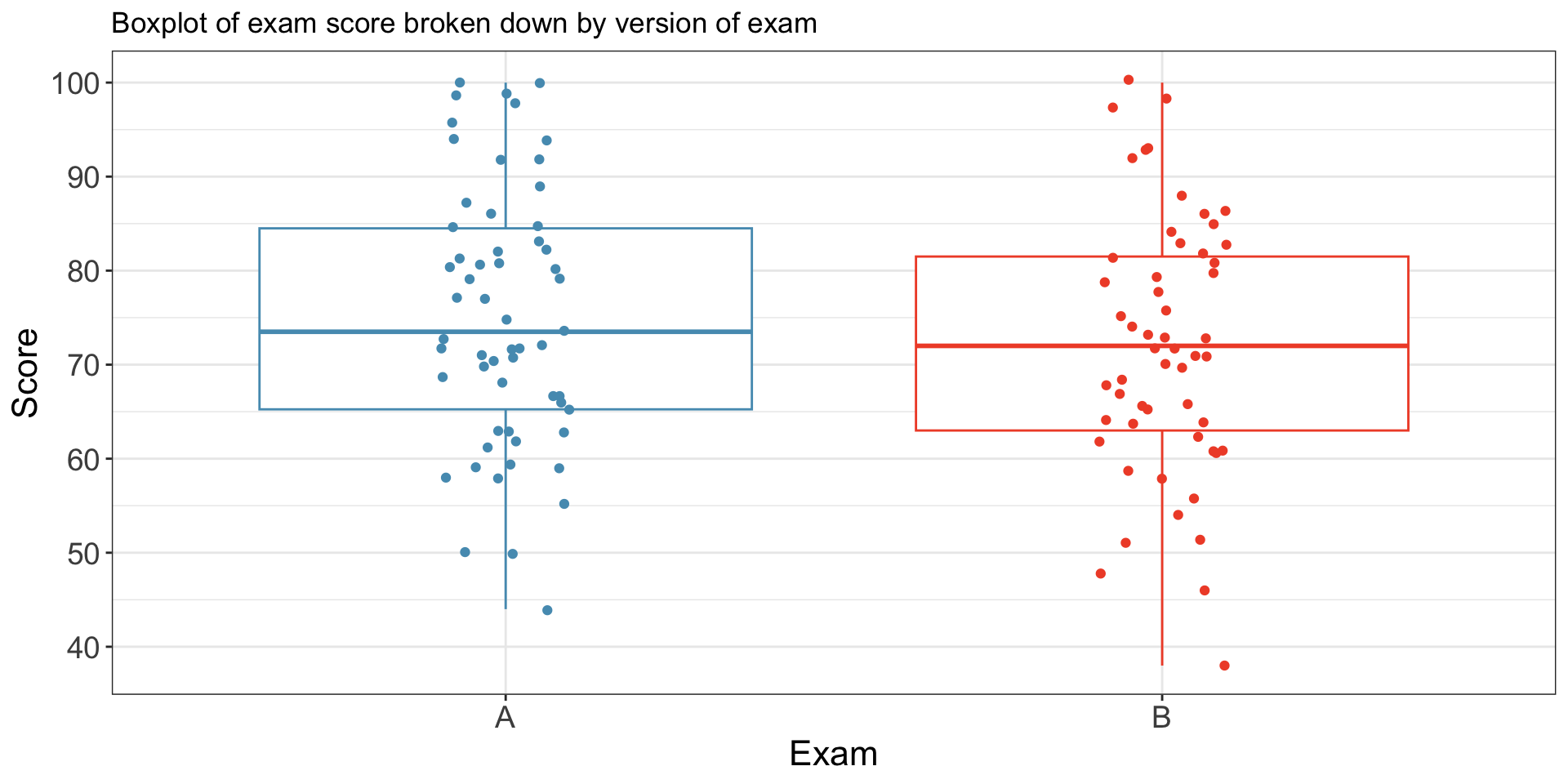
Example: Two slight variations of an exam.
- Each student received a random version (A and B).
- Anticipating complaints, the instructor wants to see if the difference observed between the groups is large enough to provide convincing evidence that one version was more difficult (on average) than the other version.
Summary statistics for how students performed on these two exams:
| Group | n | Mean | SD | Min | Max |
|---|---|---|---|---|---|
| A | 58 | 75.10 | 13.87 | 44 | 100 |
| B | 55 | 71.96 | 13.77 | 38 | 100 |
- Hypotheses to evaluate whether observed difference in sample means is likely to have happened due to chance:
- \(H_0\): exams are equally difficult; \(\mu_A = \mu_B\).
- \(H_A\): one exam is more difficult; \(\mu_A \neq \mu_B\).
- Observations regarding setup:
- Independence within each group and between groups since exams shuffled and randomly passed out.
- min/max values suggest no outliers .
- We’ll use an \(\alpha = 0.05\) discernibility threshold.
Randomization test: variability of the statistic
Previously, we estimated the variability of the proportion difference \(\hat p_1 - \hat p_2\) by randomly assigning treatment to each observation. Here we do something similar.
- To simulate the null hypothesis, we
- randomly assign 58 of the observed exam scores to group A (the remaining 55 scores then get assigned to group B), then
- examine the difference \(\bar x_{A,sim1} - \bar x_{B,sim1}\)
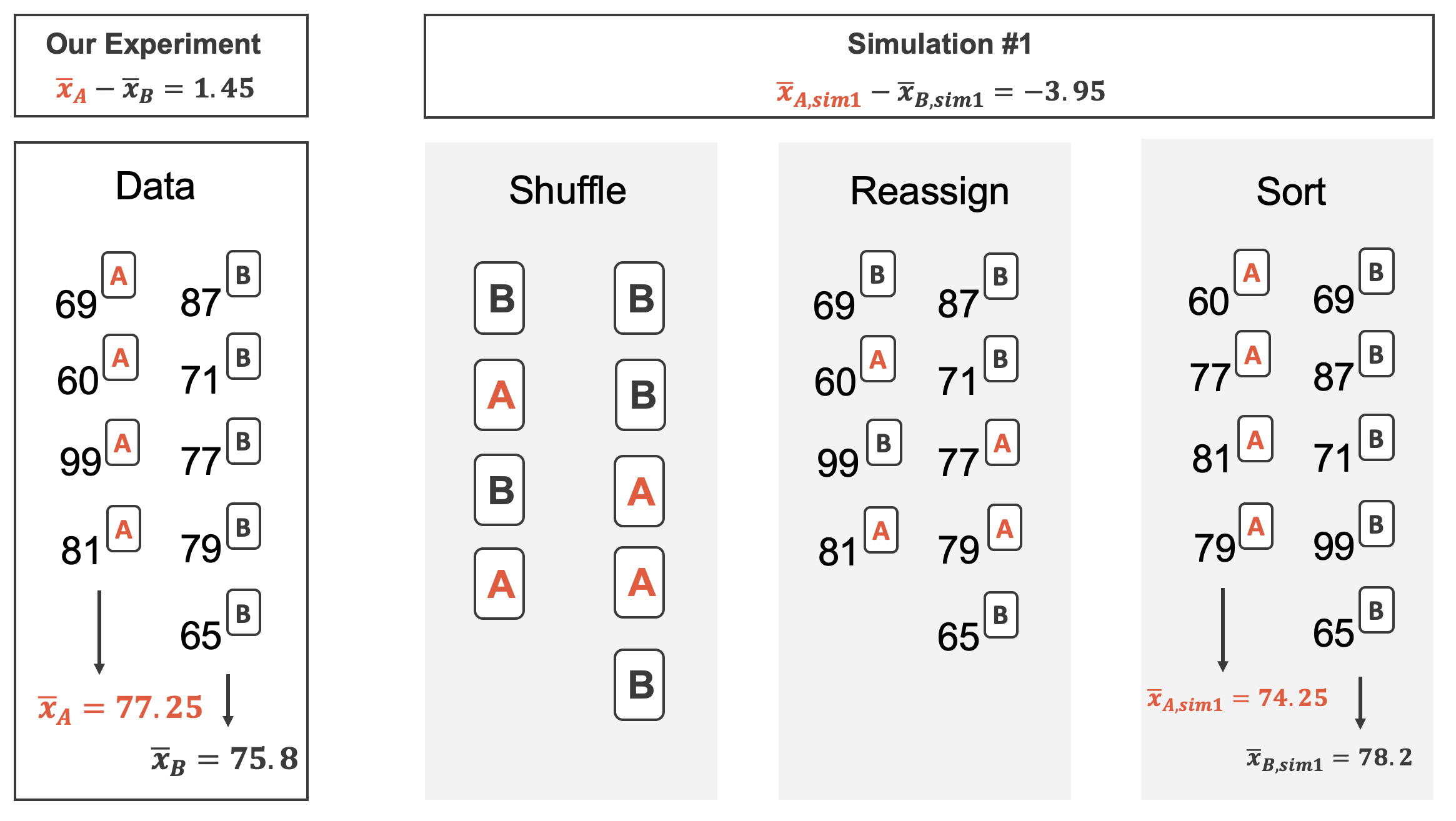
- Repeating this 10,000 times, we estimate the natural variability in \(\bar x_A - \bar x_B\) when there is no dependence between group and exam score.
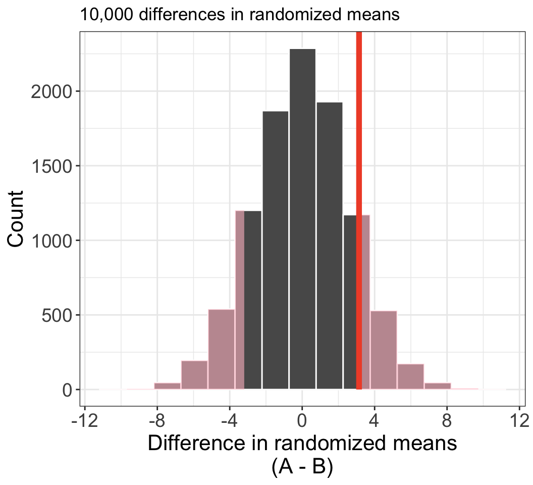
- The observed difference (highlighted above) was 75.1 - 71.96 = 3.14.
- 1195 out of 10,000 randomization trials produce a difference \(\geq\) 3.14;
- 1173 produce difference \(\leq\) -3.14.
- p-value is then \(\approx\) (1195 + 1173) / 10000 = 0.2368.
- Larger than \(\alpha = 0.05\) threshold: fail to reject \(H_0\).
- Conclude: the data do not provide enough evidence that one exam version was more difficult than the other.
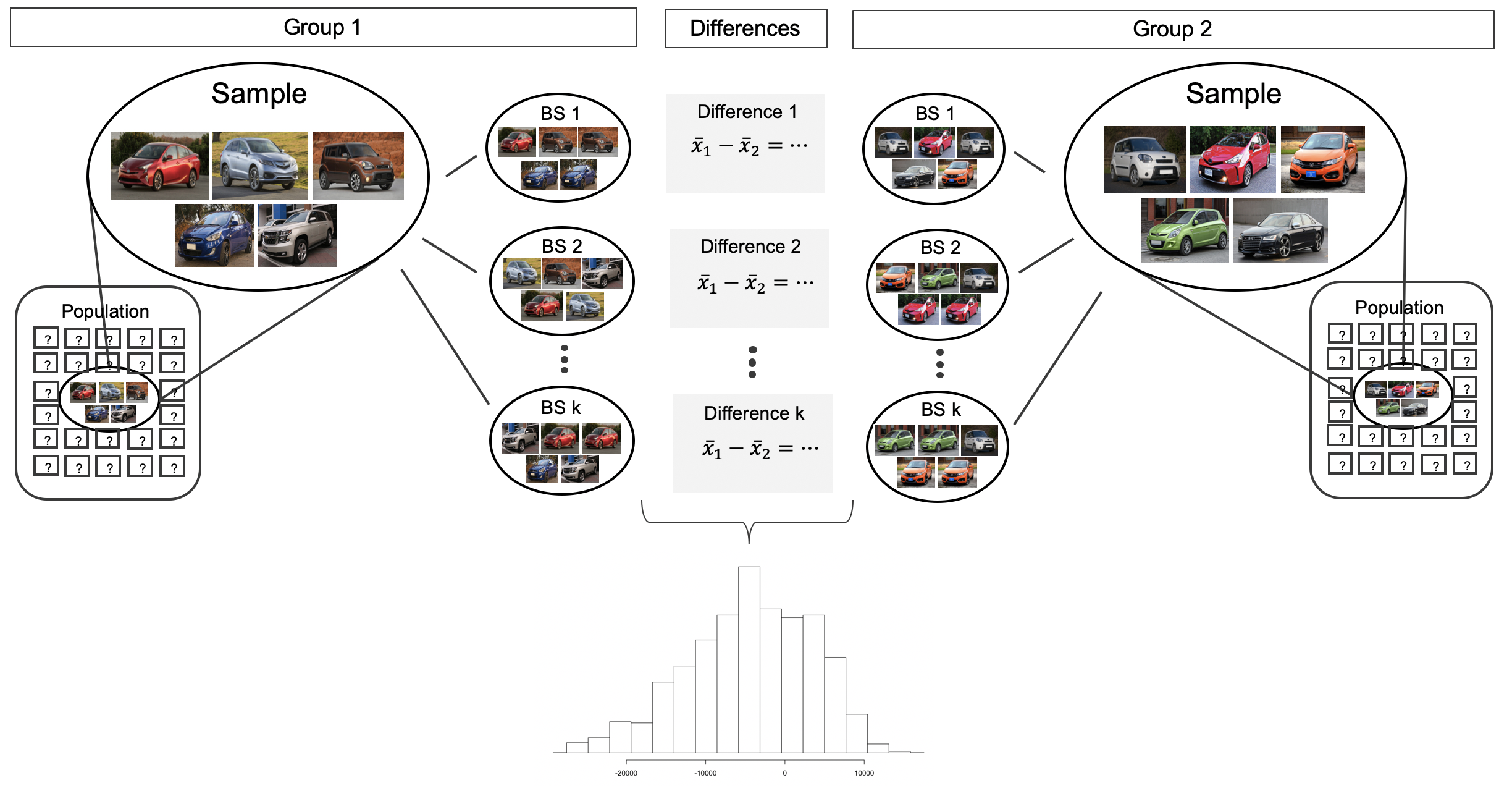
Bootstrap CI for difference in means
Example: assess 2 car lots; which one has a cheaper average price?
- We have a sample of 5 cars from each lot.
- We take bootstrap samples from each group,
- then calculate sample means in each bootstrap sample, \(\bar x_{1}^{(i)}\) and \(\bar x_{2}^{(i)}\),
- then build a distribution of the bootstrapped differences \(\bar x_{1}^{(i)} - \bar x_{2}^{(i)}\),
- then create a CI for the difference in means \(\mu_1 - \mu_2\).
Bootstrap CI: stem-cell case study
Consider the following experiment that seeks to examine whether using embryonic stem cells (ESC) help improve heart function following a heart attack
- In experiment, people are randomly assigned to treatment (ESC) and control groups, and then had their heart pumping capacity measured
- Want to compute 95% CI for effect of ESC on heart pumping capacity
- Summary statistics from experiment:
| Group | n | Mean | SD |
|---|---|---|---|
| ESC | 9 | 3.50 | 5.17 |
| Control | 9 | -4.33 | 2.76 |
- Point estimate of the difference in heart pumping capacity:
\[\bar{x}_{esc} - \bar{x}_{control}\ =\ 3.50 - (-4.33)\ =\ 7.83\]
Use bootstrap to estimate the distribution of difference in sample means when repeatedly sampling:
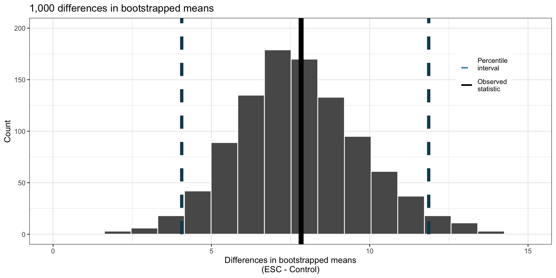
- Bootstrapped CI does not include 0.
- Conclude: ESC increases heart pumping capacity
If the CI did include 0, then we would not have enough evidence to conclude that ESC increases heart pumping capacity
- We would not say that “we have evidence that ESC does not change heart pumping capacity”.
Mathematical model for testing: Birth Weight t-test
We want to model the difference in sample means using \(t\)-distribution; check required assumptions.
- Independence: since randomly sampled, samples are independent.
- Nearly-normal data: both groups have \(>30\) observations; does data show any extreme outliers?
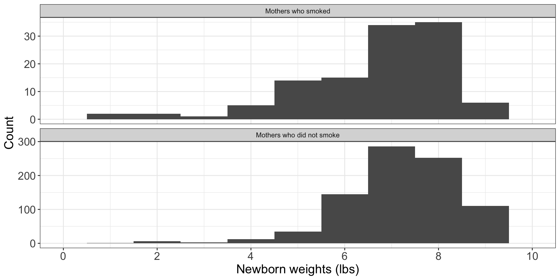
- No apparent extreme outliers, so all conditions needed to satisfy \(t\) distribution assumptions hold.
- So we can proceed with the analysis.
Let’s now complete the hypothesis test
- Let’s use \(\alpha=0.05\) (95% significance level)
- Summary statistics from before:
| Habit | n | Mean | SD |
|---|---|---|---|
| nonsmoker | 867 | 7.27 | 1.23 |
| smoker | 114 | 6.68 | 1.60 |
\[df = \min(n_1, n_2)-1 = 113\]
\[ SE \;=\; \sqrt{\frac{s_1^2}{n_1} + \frac{s_2^2}{n_2}} \;=\; \sqrt{\frac{1.23^2}{867} + \frac{1.60^2}{114}} \;=\; 0.155\] \[T \;=\; \frac{\bar x_1 - \bar x_2 - 0}{SE} \;=\; \frac{6.68-7.27}{0.155} \;=\; -3.69\]
(Street-fighting math: Before formally computing the p-value, guess whether or not we reject \(H_0\) based on the T score and df.)
- Compute the one-sided tail area:
pt(-3.69, df = 113)[1] 0.0001733097- Doubling this gives p-value of 0.00034.
- The p-value is much smaller than the significance value, 0.05, so we reject the null hypothesis \(H_0\).
- Conclude: The data provide is convincing evidence of a difference in the average weights of babies born to mothers who smoked during pregnancy and those who did not.