library(tidyverse)
library(openintro)
library(infer)

library(knitr)
library(ggpubr)
library(kableExtra)
library(gghighlight)

library(scales) # label_dollar

options(pillar.print_min = 9)  # to avoid annoying scroll behavior
knitr::opts_chunk$set(out.height = "100%")
theme_set(theme_bw() + theme(axis.text = element_text(size = 14),
                             axis.title = element_text(size = 16),
))Inference for a single mean
STA35B: Statistical Data Science 2
Bootstrap CI for a mean: in practice
If we cannot sample more from the population, we can estimate this sample-to-sample variability by bootstrapping: take \(B\) bootstrap samples of size \(n\) from the original sample of size \(n\).
- Each bootstrap sample has its own sample mean.
- There is variability across these sample means.
- This “bootstrap” variability can be an estimate for the variability of the sample mean induced by sampling repeatedly from the population.

Suppose we took 1,000 bootstrap samples, and for each bootstrap sample we compute its sample mean.
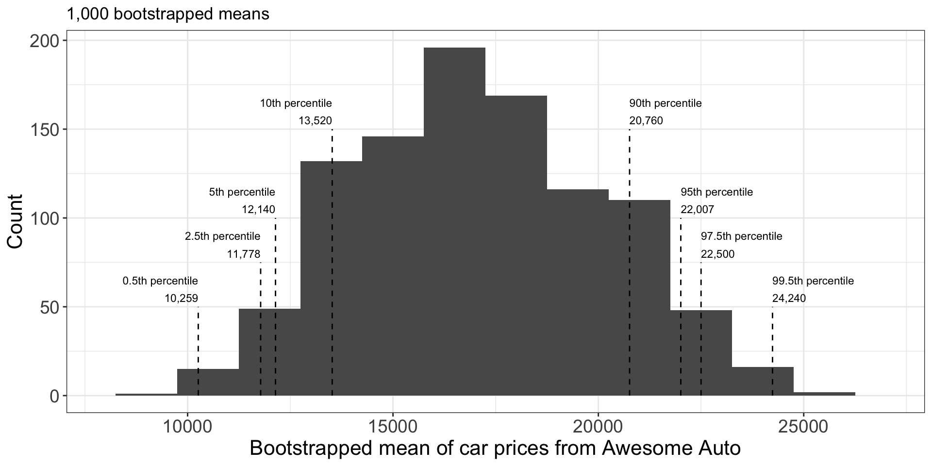
- To develop bootstrap CI for the population mean at e.g. 90% confidence level, we can calculate the 5% and 95% percentile of the bootstrapped statistics.
Let’s build a function which does the following:
- takes in a sample (a vector of numerics), and then computes a desired number of bootstrap samples and returns the means for each bootstrap sample.
boot_samp_means <- function(obs, n_resamp=10000) {
  means <- numeric(n_resamp)
  num_obs <- length(obs)
  for(i in 1:n_resamp) {
    resampled <- sample(obs, size=num_obs, replace=TRUE)
    means[i] <- mean(resampled, na.rm=TRUE)
  }
  return(means)
}
or
boot_samp_means <- function(obs, n_resamp=10000) {
  num_obs <- length(obs)
  replicate(
      n_resamp,
      sample(obs, size=num_obs, replace=TRUE) |> mean(na.rm=TRUE)
      )
}- For the car example, here’s how we could do this:
obs <- c(18300, 20100, 9600, 10700, 27000)
mean(obs)
[1] 17140bs_means <- boot_samp_means(obs, 10000)
str(bs_means) num [1:10000] 13300 17360 16560 20620 22360 ...- To construct a 90% CI, find 5th percentile and 95th percentile.
(qs <- quantile(bs_means, probs=c(0.05, 0.95))) 5% 95%
12140 22140 - We are 90% confident that the true average is between $12140 and $22140.
Bootstrap CI for a standard deviation: car
Results of bootstrap standard deviations:
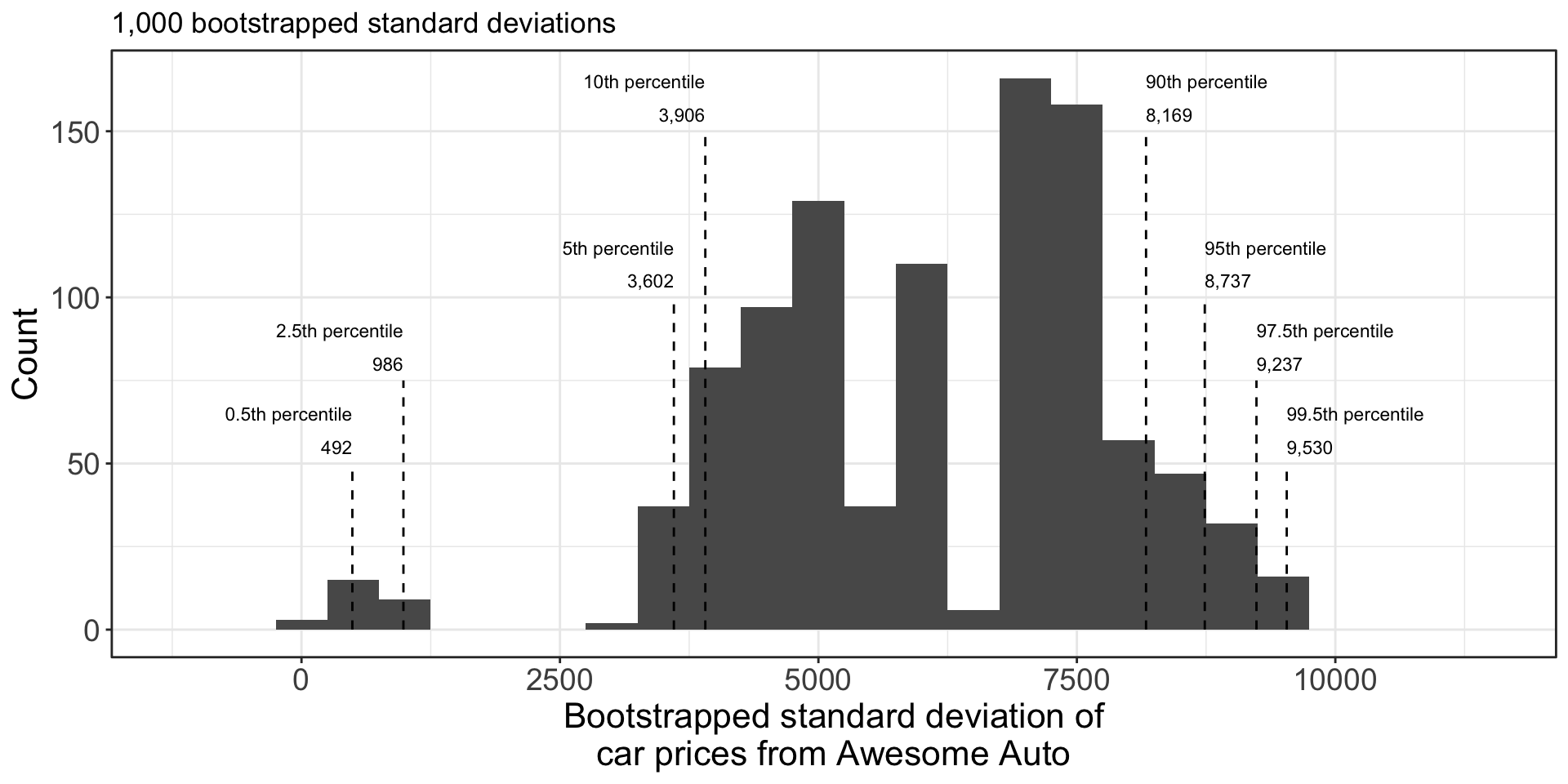
- Very high variability. This is due to the tiny sample size - only 5 observations.
- As we increase the original dataset sample size, the bootstrap improves.
- A precise characterization of how sample size / number bootstrap trials affect the accuracy of the bootstrap is beyond this course. (It is still the subject of current research.)
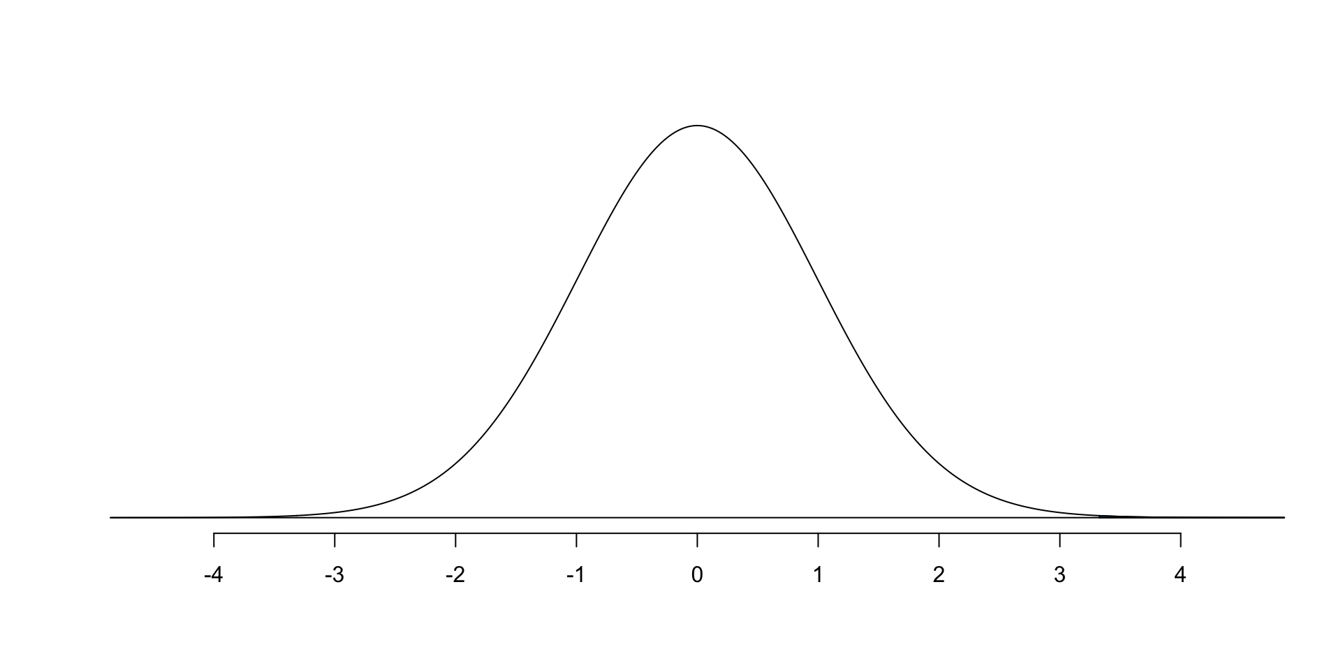
\(t\) distribution
- The \(t\) distribution is defined in terms of degrees of freedom
df. - Has a similar bell-shaped curve to normal, but has “thicker tails”, which allows for more extreme events to occur than in a normal distribution.
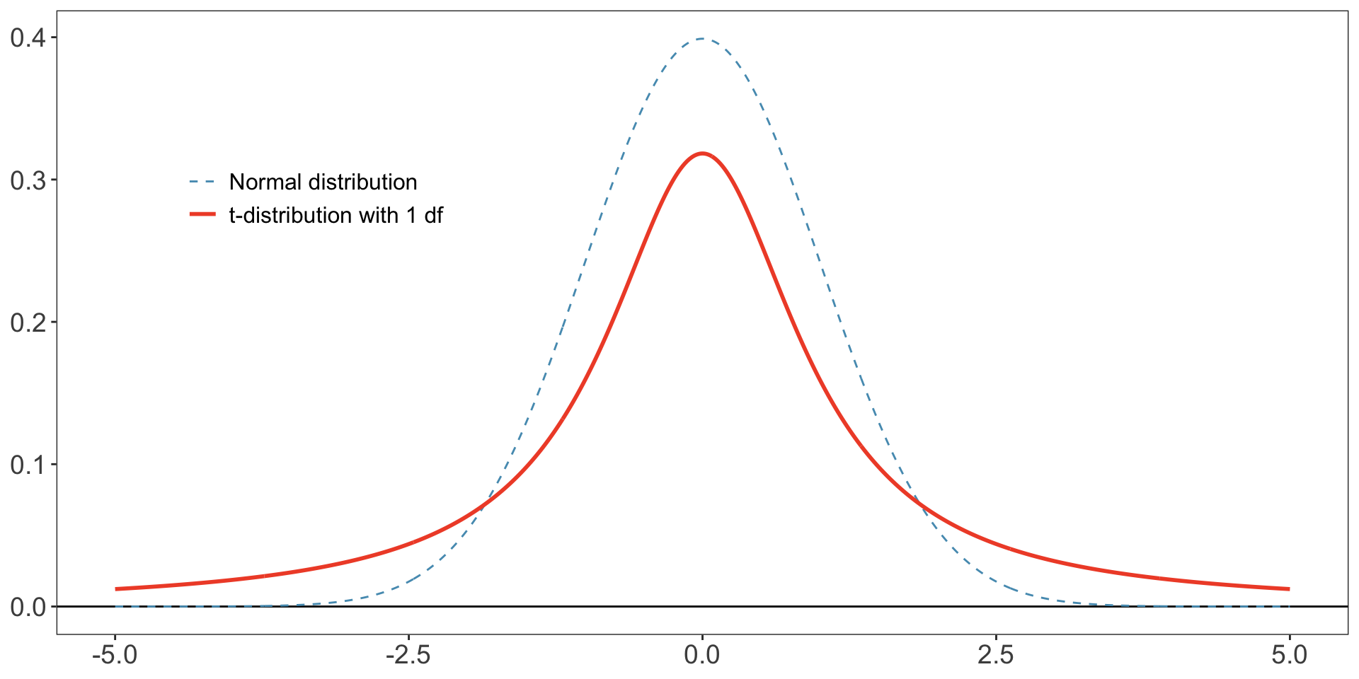
- Data from a normal distribution has very little data beyond 2.5;
- Data from a \(t\) distribution has relatively more, particularly when df is small.
Effect of df on \(t\) distribution:
- Given data with \(n\) samples, we will typically use \(t\) distribution with \(n-1\) df.
- Few samples: more uncertainty when estimating population’s variance.
- Many samples: less uncertainty when estimating population’s variance.
- As df increases, the \(t\) distribution gets thinner tails and increasingly resembles a standard normal.
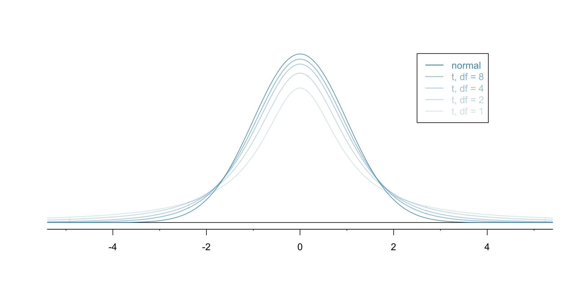
- When df \(>30\), almost indistinguishable from standard normal.
- Intuition: height/thickness represents how likely values are; when df (\(n-1\)) is small, we are more uncertain and so more extreme values are more likely.
\(t\) distribution: example calculations I
- Probability that \(t\) distribution with 20 degrees of freedom is less than -1.5?
# use pt() to find probability
# under the $t$-distribution
pt(-1.5, df = 20)
[1] 0.07461789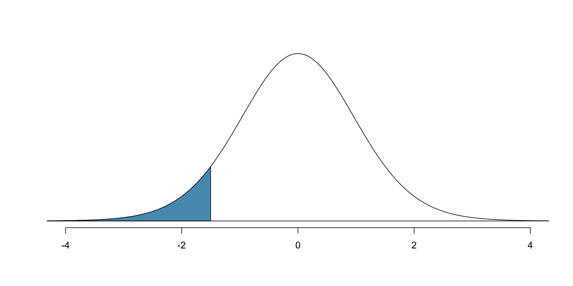
- Probability that \(t\) distribution with 11 degrees of freedom is bigger than 2.5?
1 - pt(2.5, df = 11)[1] 0.01475319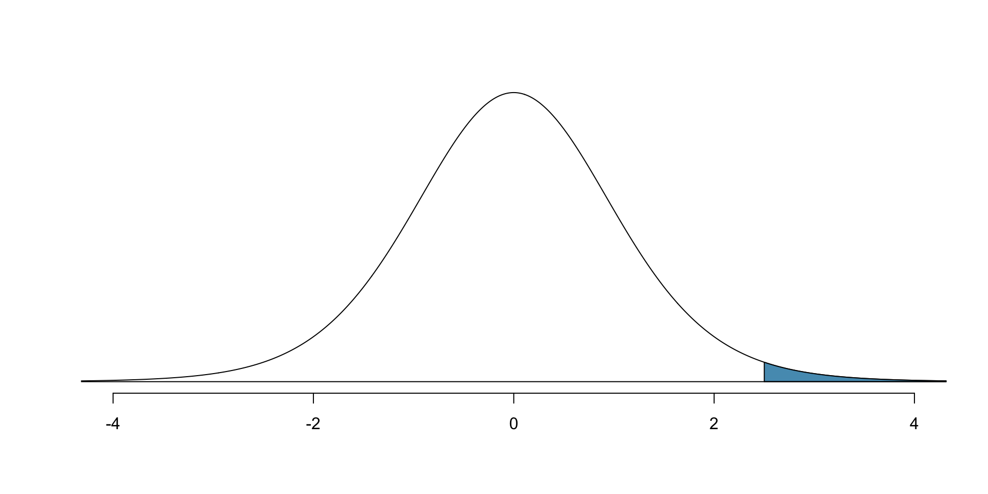
\(t\) distribution: example calculations II
Probability that \(t\) distr. with 2 df is more than 3 units away from the mean?
# use pt() to find probability under the $t$-distribution
pt(-3, df = 2) + (1 - pt(3, df = 2))
[1] 0.09546597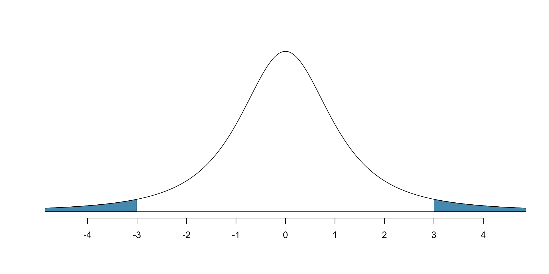
- Any \(t\) distribution is symmetric around 0, so…
2*pt(-3, df = 2) # ...could also do this[1] 0.09546597- Compare with what happens with standard normal: 68-95-99.7 rule says that only 0.3% (=0.003) would be more than 3 units from the mean.
- Since \(t\) distribution has fatter tails, it assigns greater probability to extreme values, so we get significantly more area for \(t\) distribution.
- As degrees of freedom increase, this becomes less and less the case.
One-sample \(t\)-distribution CI: calculation
- Same idea holds for finding \(t^*_{df}\): to get confidence level of \(1-\alpha\), we use
qt(1 - alpha/2, df = df)
- E.g. if df = 5 and we want 95% confidence level,
qt(1 - 0.05/2, df = 5)[1] 2.570582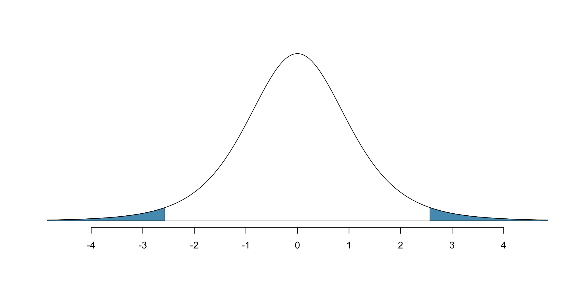
- E.g. if df = 10 and we want 95% confidence level,
qt(1 - 0.05/2, df = 10)[1] 2.228139- E.g. if df = 50 and we want 95% confidence level,
qt(1 - 0.05/2, df = 50)[1] 2.008559- E.g. if df = 500 and we want 95% confidence level,
qt(1 - 0.05/2, df = 500)[1] 1.96472- E.g. if df = 5000 and we want 95% confidence level,
qt(1 - 0.05/2, df = 5000)[1] 1.960439- As df increases, the t-distribution’s critical value seems to be approaching
qnorm(1 - 0.05/2)[1] 1.959964One sample \(t\)-test: Cherry Blossom
Are runners in Washington, DC races are getting slower or faster over time?
- In 2006, DC Cherry Blossom Race (10 miles) had average of 93.29 minutes
- Will use data from 100 participants from 2017 to determine whether runners are getting faster or slower (vs. possiblity of no change)
- \(H_0\): average 10 mile time is same in 2006 as in 2017, so \(\mu = 93.29\)
- \(H_A\): average 10 mile run time is different in 2017; \(\mu \neq 93.29\)
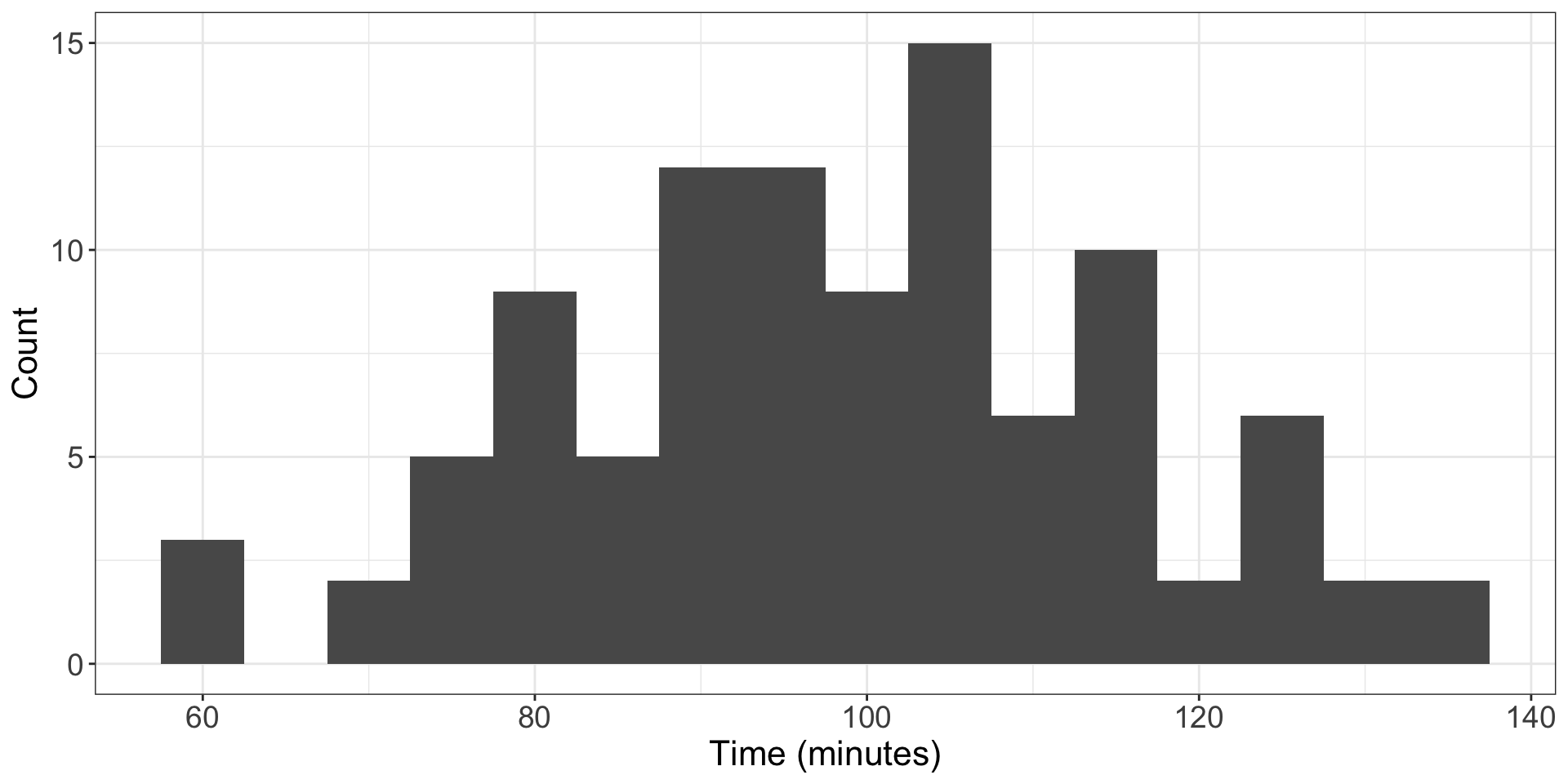
- Data looks like:
Large enough samples, no extreme outliers, can proceed
To do the hypothesis test, same procedure as before
- Normal setting: find Z-score using observed value, null value, standard error, then use normal distribution to calculate tail area / p value
- This setting: T-score using observed value, null value, standard error, then use t distribution to calculate tail area / p value
For sample of 100 runners, 2017 data had average of 98.78 and s.d. of 16.59; average run time in 2006 was 93.29
First calculate standard error:
\[ SE = \frac{s}{\sqrt{n}} = \frac{16.59}{\sqrt{100}} = 1.66\]
- T score:
\[ T = \frac{\text{observed}-\text{null}}{SE} = \frac{98.8 - 93.29}{1.66} = 3.32\]
- We have \(n=100\) observations, so \(df=100-1=99\).
- We can use
ptto find this; by symmetry, area to right of 3.32 is same as area to left of -3.32, so
pt(-3.32, df = 99)[1] 0.0006305322- Double this to get the p-value: 0.00126.
- \(p\)-value is \(<0.05\), so we can reject the null hypothesis at 95% confidence level.
- Can reject at even 99% confidence level.
- Thus average run time in 2017 is different than 2006.