Inference for two proportions

STA35B: Statistical Data Science 2

Akira Horiguchi

Based on Ch 17 of IMS

library(tidyverse)
library(openintro)
library(infer)

library(knitr)
library(ggpubr)
library(kableExtra)
library(gghighlight)

library(scales) # label_dollar

options(pillar.print_min = 9)  # to avoid annoying scroll behavior
knitr::opts_chunk$set(out.height = "100%")
theme_set(theme_bw() + theme(axis.text = element_text(size = 14), 
                             axis.title = element_text(size = 16), 
                             ))

Overview

Derive confidence intervals and hypothesis tests for differences in population proportions from two groups: \[p_1 - p_2.\]

  • We will estimate \(p_1-p_2\) by \(\hat p_1 - \hat p_2\).
    • \(\hat p_1\) = observed proportion of successes in group 1.
    • \(\hat p_2\) = observed proportion of successes in group 2.
  • To estimate variability / perform inference, we’ll use three methods:
    • Randomization test
    • Bootstrap for confidence intervals
    • Normal approximation

CPR Survival Experiment

Patients underwent CPR for a heart attack and then admitted to a hospital.

  • Patients are randomly assigned to either receive blood thinner (treatment) or not (control)
  • Outcome: whether patient survived for at least 24 hours after heart attack.
str(openintro::cpr)
tibble [90 × 2] (S3: tbl_df/tbl/data.frame)
 $ group  : Factor w/ 2 levels "control","treatment": 1 1 1 1 1 1 1 1 1 1 ...
 $ outcome: Factor w/ 2 levels "died","survived": 2 2 2 2 2 2 2 2 2 2 ...
Group Died Survived Total
Control 39 11 50
Treatment 26 14 40
Total 65 25 90
  • Proportion of treatment patients who survive: \(\hat p_T = \frac{14}{40} = 0.35\)
  • Proportion of control patients who survive: \(\hat p_C = \frac{11}{50} = 0.22\)
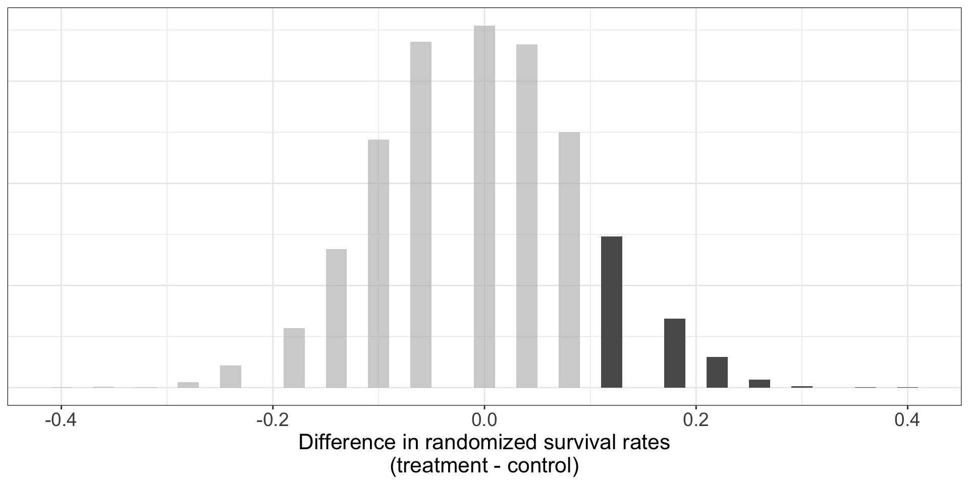
  • How likely would observed \(\hat p_T - \hat p_C = 0.13\) occur due to random chance?

Randomization test

Formulate a hypothesis test:

  • \(H_0\): blood thinners after CPR is independent of survival: \(p_1-p_2=0\).
  • \(H_A\): blood thinners after CPR increase chance of survival: \(p_1-p_2>0\).

Since initial assignment of treatment/control was random, if we reject the null, we can say that difference was due to usage of blood thinners (causal claim).

Randomization procedure

  • Assume that the same number of people died (65) / survived (25).
  • Then see what happens if we randomly assign treatment or control to each.
  • For \(i\)th simulated treatment/control group, calculate proportion \(\hat p_{1}^{(i)} - \hat p_{2}^{(i)}\).
Figure 1: Histogram of 10000 simulated proportion differences.
  • 1279/10000 simulations had a difference of \(\geq 13\%\).
  • This implies about 12% chance of differences like we saw if \(H_0\) were true.
  • Under significance level \(\alpha = 0.05\), we will not reject \(H_0\): not enough evidence to claim that blood thinners improve survival rate.

Bootstrap confidence interval for difference in proportions

We can also perform inference on \(p_1-p_2\) by constructing a bootstrap CI.

  • We previously applied bootstrap sampling to a single population.
  • We now have samples from two different groups:
    • Resample from group 1 to calculate \(\hat p_{1}^{(i)}\).
    • Resample from group 2 to calculate \(\hat p_{2}^{(i)}\).
Figure 2: Cartoon of bootstrap samples with two groups.
  • Each pair of bootstrap samples gives us an estimate \(\hat p_{1}^{(i)} - \hat p_{2}^{(i)}\).
  • We can use this to create a distribution of the difference in proportions.

Bootstrap confidence interval: result

Figure 3: Histogram of 10000 bootstrapped proportion differences.

For a 95% CI, we want to find the 2.5th and 97.5th percentiles/quantile:

CI95 <- quantile(cpr_boot_dist$stat, c(0.025, 0.975))
  • The 95% CI is then (-0.059, 0.318).
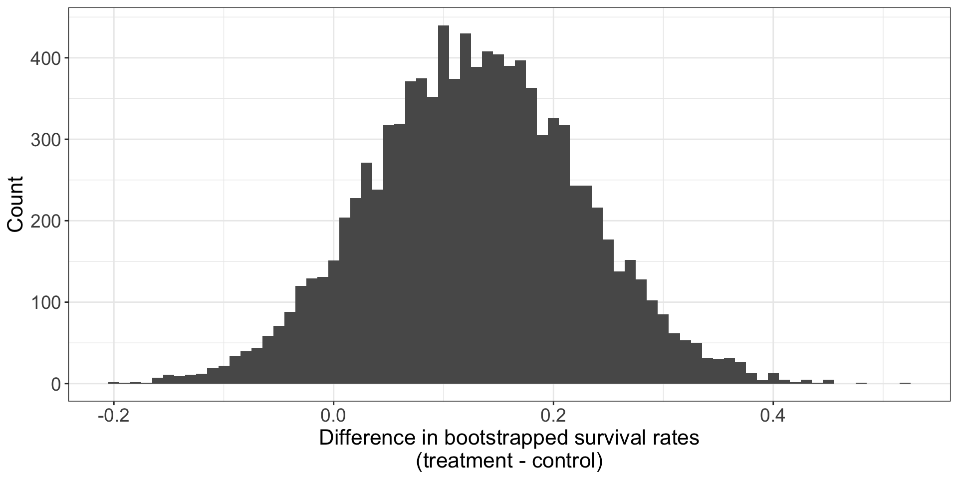
  • 95% confidence that in the population, the true difference in survival rate for people receiving blood thinners post CPR is between 0.059 lower and 0.318 higher than the survival rate for non-receivers.

Similar calculation for 90% CI (which will be a narrower interval):

CI90 <- quantile(cpr_boot_dist$stat, c(0.05, 0.95))
  • Even the 90% CI (-0.03, 0.288) still includes 0.

Mathematical model for difference in proportions

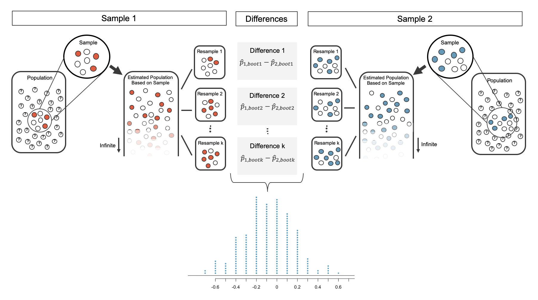
Like with \(\hat p\) for a single proportion, the difference \(\hat p_1 - \hat p_2\) can be modeled with a normal distribution under certain (more stringent) assumptions:

  • Independence: data within each group and between groups are independent; generally satisfied if in randomized experiment.
  • Success-failure: at least 10 successes and 10 failures within each group.

When these conditions are satisfied, the standard error of \(\hat p_1 - \hat p_2\) is

\[SE(\hat{p}_1 - \hat{p}_2) = \sqrt{\frac{p_1(1-p_1)}{n_1} + \frac{p_2(1-p_2)}{n_2}}\]

  • \(p_1\) and \(p_2\) are the population proportions; \(n_1\) and \(n_2\) are the sample sizes.

In most cases, the standard error is approximated using the observed data:

\[\sqrt{\frac{\hat{p}_1(1-\hat{p}_1)}{n_1} + \frac{\hat{p}_2(1-\hat{p}_2)}{n_2}}\]

  • \(\hat{p}_1\) and \(\hat{p}_2\) represent the observed sample proportions.

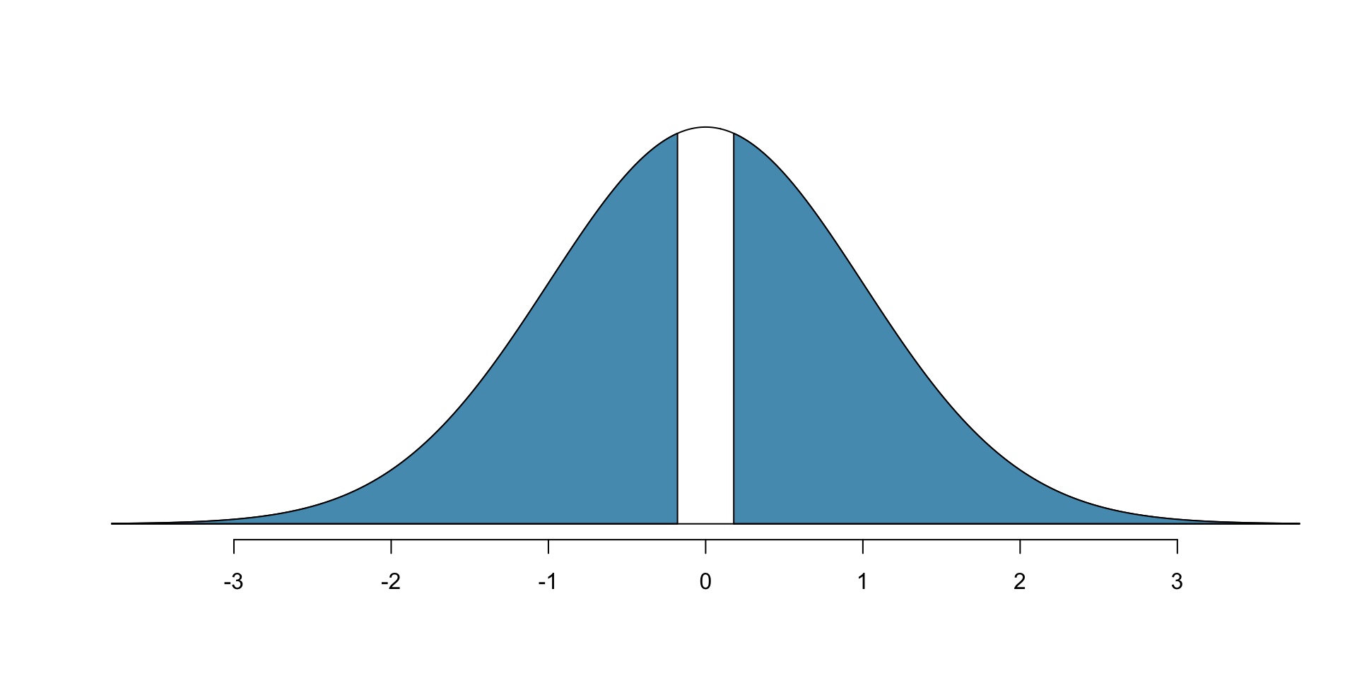
Margin of error is defined in terms of standard error: \[z^\star \times \sqrt{\frac{\hat{p}_1(1-\hat{p}_1)}{n_1} + \frac{\hat{p}_2(1-\hat{p}_2)}{n_2}}.\]

  • \(z^\star\) is calculated from a specified percentile on the normal distribution (e.g. 1.96 for 95%).

Can then use standard approach for defining a CI:

\[ \begin{aligned} \text{point estimate} \ &\pm \ z^{\star} \ \times \ SE \\ (\hat{p}_1 - \hat{p}_2) \ &\pm \ z^{\star} \times \sqrt{\frac{\hat{p}_1(1-\hat{p}_1)}{n_1} + \frac{\hat{p}_2(1-\hat{p}_2)}{n_2}} \end{aligned} \]

Mathematical model: CPR dataset

Are conditions met?

  • Random assignment of treatment/control, so independence is satisfied
  • Success-failure condition in each group: 11, 14, 39, 26 in each outcome, so condition is satisfied.
Group Died Survived Total
Control 39 11 50
Treatment 26 14 40
Total 65 25 90

Let’s create a 90% CI for difference in survival rates.

  • Point estimate:

\[\hat{p}_{T} - \hat{p}_{C} = \frac{14}{40} - \frac{11}{50} = 0.35 - 0.22 = 0.13\]

  • Formula for the SE:

\[SE \approx \sqrt{\frac{0.35 (1 - 0.35)}{40} + \frac{0.22 (1 - 0.22)}{50}} = 0.095\]

  • Need to find \(z^*\) for 90% confidence interval:
qnorm(0.05)
[1] -1.644854
  • \(z^* = 1.64\), so

\[ \begin{aligned} \text{point estimate} \ &\pm \ z^{\star} \ \times \ SE \\ 0.13 \ &\pm \ 1.64 \ \times \ 0.095 \\ (-0.027 \ &, \ 0.287) \end{aligned} \]

Conclusion: We are 90% confident that individuals receiving blood thinners have between a 2.7% smaller chance of survival to 28.7% greater chance of survival.

  • Since 0% is in the interval, we cannot conclude that blood thinners have an effect on CPR.
  • Close to bootstrap estimate for 90% CI, (-0.03, 0.288), so same conclusion.
    • (The slight differences come from approximation error from simulations for bootstrap and from mathematical approximation.)
  • Similarly, using randomization test, we found around 12% likelihood that difference we observed in the original dataset (13%) would occur due to random chance if blood thinner treatment is independent of survival.

Hypothesis test

For hypothesis test for difference in proportions being not equal (null \(H_0\): \(p_1-p_2=0\)), similar ideas from before: calculate SE and check technical conditions like independence and success-failure.

  • One difference: success-failure is defined in terms of pooled proportion, \[ \hat p_{pool} = \frac{\text{number successes}}{\text{number cases}} = \frac{\hat p_1 n_1 + \hat p_2 n_2}{n_1 + n_2}. \] Note that \[ \hat p_1 = \frac{\text{number successes in sample 1}}{n_1}.\]

  • From this we can formulate a test statistic for assessing difference in two proportions - a Z score

  • Standard error: approximation for the standard deviation of the sampling distribution for \(\hat p_1 - \hat p_2\) \[\sqrt{\hat p_{pool}(1-\hat p_{pool}) \left( \frac{1}{n_1} + \frac{1}{n_2}\right)}\]

  • General form for Z-score:

\[ \begin{align*} Z &= \frac{\text{point estimate} - \text{null value}}{SE} \\ &= \frac{\hat p_1 - \hat p_2 - 0}{ \sqrt{\hat p_{pool}(1-\hat p_{pool}) \left( \frac{1}{n_1} + \frac{1}{n_2}\right) }} \end{align*} \]

  • When \(H_0\) is true and following conditions hold, \(Z\) has approximately standard normal distribution.
    • Independent observations
    • Sufficiently large samples:
      \(n_1\,\hat p_{pool} \geq 10, \quad n_1 (1-\hat p_{pool}) \geq 10,\)
      \(n_2\,\hat p_{pool} \geq 10, \quad n_2 (1-\hat p_{pool}) \geq 10\)

Mammogram study

We’ll look at data for whether getting mammograms as a part of regular breast cancer exams is effective at reducing death from breast cancer.

  • Control: non-mammogram breast cancer exam.
  • Treatment mammograms included in breast cancer exam.

Randomly assigned ~90,000 people to each of control/treatment groups.

  • mammogram dataset from openintro package
Death from breast cancer?
Treatment Yes No
control 505 44,405
mammogram 500 44,425

We want to test whether mammograms are effective

  • Formulate hypotheses:
    • \(H_0\): mammograms do not affect survival likelihood (\(p_M = p_C\))
    • \(H_A\): mammograms improve likelihood of survival (\(p_M > p_C\))
  • Check conditions for being able to use Z-score:
    • Indep: random treatment assignment
    • Success-failure: need to calculate \(\hat p_{pool}\), \[\begin{align} \hat p_{pool} &= \frac{\text{# of patients died from breast cancer}}{\text{# of patients in study}} \\ &= \frac{500 + 505}{500 + 44425 + 505 + 44405} = 0.0112 \end{align}\] \[ \begin{align*} \hat{p}_{\textit{pool}} \times n_{M} &= 0.0112 \times \text{44,925} = 503\\ (1 - \hat{p}_{\textit{pool}}) \times n_{M} &= 0.9888 \times \text{44,925} = \text{44,422} \\ \hat{p}_{\textit{pool}} \times n_{C} &= 0.0112 \times \text{44,910} = 503\\ (1 - \hat{p}_{\textit{pool}}) \times n_{C} &= 0.9888 \times \text{44,910} = \text{44,407} \end{align*} \] - All are at least 10
      • Z score is approximately standard normal

Mammogram Test Statistic

Death from breast cancer?
Treatment Yes No
control 505 44,405
mammogram 500 44,425
  • To calculate a confidence interval, we need the point estimate as well as the standard error
  • \(\hat p_{pool} = 0.0112\) is our best estimate of \(p_M\) and \(p_C\) if the null hypothesis is true that \(p_M = p_C\); we will use this to compute the standard error

The breast cancer death rate in the mammogram group was 0.012% less than in the control group. Next, the standard error is calculated using the pooled proportion \(\hat{p}_{\textit{pool}}:\)

\[\hat{p}_{M} - \hat{p}_{C}= \frac{500}{500 + 44425} - \frac{505}{505 + 44405} = -0.00012\]

\[SE = \sqrt{\frac{\hat{p}_{\textit{pool}}(1-\hat{p}_{\textit{pool}})}{n_{M}} + \frac{\hat{p}_{\textit{pool}}(1-\hat{p}_{\textit{pool}})}{n_{C}}}= 0.00070\]

Just like in past tests, we first compute a test statistic and draw a picture:

\[Z = \frac{\text{point est} - \text{null val}}{SE} = \frac{-0.00012 - 0}{0.00070} = -0.17\]

  • Z score: -0.17
  • Right tail area: 0.4325, via pnorm(-0.17).
  • Double to get the p-value: 0.8650
  • Can we conclude mammograms have no benefits or do not cause harm?
    • We do not reject the null given the evidence — if mammograms help or hurt, the data suggests the effect is not too large.
    • We do not “accept” the null hypothesis — we just do not have enough evidence to reject it.