Inference for a single proportion

STA35B: Statistical Data Science 2

Akira Horiguchi

Based on Ch 16 of IMS

library(tidyverse)
library(openintro)
library(infer)

library(knitr)
library(ggpubr)
library(kableExtra)
library(gghighlight)

library(scales) # label_dollar

options(pillar.print_min = 9)  # to avoid annoying scroll behavior
knitr::opts_chunk$set(out.height = "100%")
theme_set(theme_bw() + theme(axis.text = element_text(size = 14), 
                             axis.title = element_text(size = 16), 
                             ))

A more thorough treatment of inference for proportions

In this setting, for each observation there is only a single (categorical) variable taking one of two values measuring success or failure

e.g. “surgical complication” or “no complication”.
Since there’s only a single variable, we cannot do a randomization test.
We resort to bootstrapping and mathematical models.

Let’s return to the medical consultant example

A consultant tries to attract patients by saying that only 3 of her 62 clients (4.8%) had complications from surgeries; baseline US average complication rate is 10%.

Was not a randomized trial, so no way to assess whether her actions cause lower complication rate (she could have selectively chosen healthy patients).
However, we can assess whether the observed proportion $\hat p = \frac{3}{62} \approx 0.048$ would occur due to random chance given population average of $p_0 = 0.1$.
Can formulate this as a hypothesis test:
- $H_0$: no association between consultant contributions and complication rate; $p=0.10$
- $H_A$: patients with consultant associated with lower complication rate; $p<0.10$
We’ll estimate a “p-value”: if the null hypothesis is true, what is the probability of observing a test statistic $(\hat p)$ that is as extreme as the one we saw?

Sampling under the null hypothesis

What is the sampling distribution of the test statistic $\hat p$ if $H_0$ is true?

Dataset: 3 of 62 donors had complications.
Under $H_0$, 10% of donors have complications.
Now we want to simulate additional datasets of size 62, where with probability 10%, the donor has a complication.
$i$th simulated dataset will produce a proportion $\hat{p}_{sim}^{(i)} = \frac{\# \text{ complications}}{62}$

set.seed(37)
comp_rate_obs <- 3/62
medical_consultant_sim_dist <- tibble(stat = rbinom(10000, 62, 0.1)/62)

medical_consultant_n_sim <- medical_consultant_sim_dist |>
  filter(stat <= comp_rate_obs) |>
  nrow()

medical_consultant_p_val <- round(medical_consultant_n_sim / 10000, 3)

ggplot(medical_consultant_sim_dist, aes(x = stat)) +
  geom_histogram(binwidth = 0.0167) +
  gghighlight(stat <= comp_rate_obs) +
  scale_x_continuous(breaks = seq(0, 0.5, 0.02), labels = label_number(accuracy = 0.01)) +
  labs(
    x = expression(hat(p)[sim]),
    y = "Number of simulated scenarios"
  )

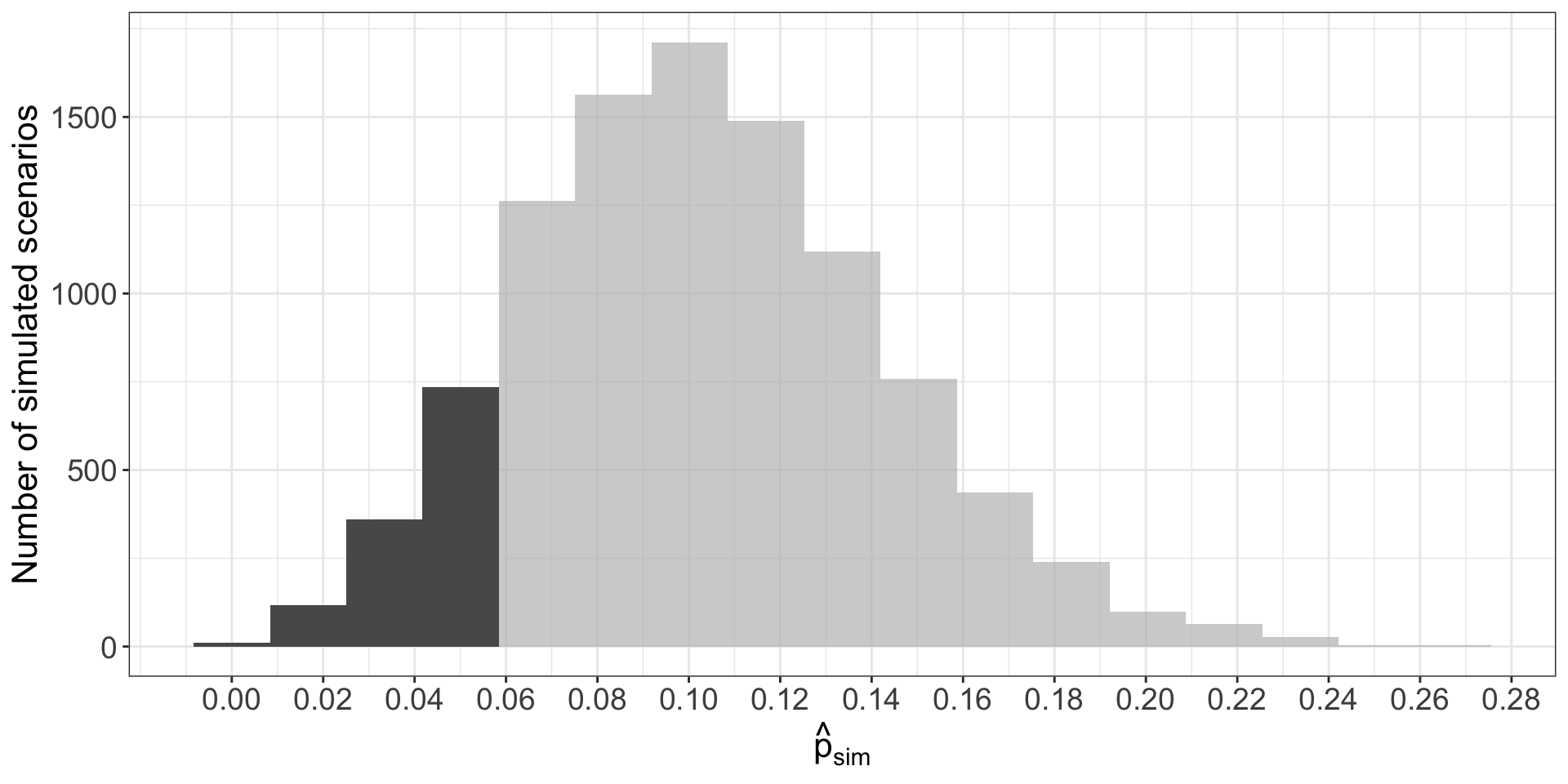
Histogram of simulated proportions for 10000 simulated datasets. Shaded = sample proportions under null that are as extreme as the observed 3/62.

1222 simulated sample proportions were $\leq 3/62$
We use these to construct the null distribution’s left-tail area:

\[\begin{align*} \text{left area} = \frac{\text{# sims w/ }\hat{p}_{sim}^{(i)} \leq \text{ (3/62)}}{\text{total # sims}} \end{align*}\]

Our estimated p-value is equal to this tail area: 0.122.

How do we do this binomial simulation in R?

Each bootstrap sample (size $n=62$) had its own proportion of succcesses \[\begin{align*} \hat p_{sim}^{(i)} = \frac{\text{# complications in $i$th sample}}{n}. \end{align*}\]
Each donor had a probability $p$ of having a complication.
Then the $\#$ of complications follows a binomial distribution with parameters $n=62$ and $p=0.1$. This is denoted as Binomial(n,p).

More generally, Binomial(n,p) models the number of successes in $n$ independent trials when each trial has probability $p$ of success.

To create the 10,000 bootstrap proportions, use: rbinom(10000, n, p)
- This generates a vector of length 10000, where each component is the outcome of n where probability of success in each trial is p

To convert number of successes to proportion, need to divide by $\#$ of trials

n_successes <- rbinom(10000, 62, 0.1)
tibble(stat = n_successes / 62)

# A tibble: 10,000 × 1
    stat
   <dbl>
1 0.129 
2 0.145 
3 0.0968
4 0.113 
5 0.129 
6 0.0323
7 0.0645
8 0.0968
9 0.0968
# ℹ 9,991 more rows

Mathematical model

The sampling distribution for $\hat{p}$ based on a sample of size $n$ from a population with a true proportion $p$ is nearly normal when:

The sample’s observations are independent, e.g., are from a simple random sample.
We expected to see at least 10 successes and 10 failures in the sample, i.e., $np\geq10$ and $n(1-p)\geq10.$ This is called the success-failure condition.

When both conditions are met, then the sampling distribution of $\hat{p}$ is nearly normal with mean $p$ and standard error of $\hat{p}$ as $SE(\hat{p}) = \sqrt{\frac{\ p(1-p)\ }{n}}.$

Checking the two conditions

The independence condition is a more nuanced requirement (outside the scope of this class).
How do we check the success-failure condition when typically we don’t know the true proportion $p$? We can estimate $p$ with either…
- …the sample proportion $\hat{p}$, if computing confidence intervals;
- …the null value $p_0$, if performing a hypothesis test.

Confidence interval

Provides a range of plausible values for proportion $p$

When the sample proportion $\hat{p}$ can be modeled using a normal distribution, a confidence interval for proportion $p$ takes the form \[\begin{align*} \hat p \pm z^* \times SE(\hat{p}) \end{align*}\] where \[\begin{align*} SE(\hat p) = \sqrt{\frac{p(1-p)}n}. \end{align*}\]
Since $p$ is unknown, we typically use \[\begin{align*} SE(\hat{p}) \approx \sqrt{\frac{(\mbox{best guess of }p)(1 - \mbox{best guess of }p)}{n}} \end{align*}\]
$z^*$ is a threshold depending upon level of confidence desired $(z^*=1.96$: 95% level)

Example: random sample of 826 payday loan borrowers, assessing interest in regulation for payday loans. 70% of responders say they support regulations.

Is it reasonable to model the sample-to-sample variability of $\hat{p}$ using a normal distribution?
Estimate the standard error of $\hat{p}.$
Construct a 95% confidence interval for $p,$ the proportion of payday borrowers who support increased regulation for payday lenders.

Confidence interval example solution

Data are a random sample, so reasonable to assume independent observations that represent the population. Need to check success-failure condition. We don’t have $p$, so have to use $\hat p$ to estimate it:
- $\text{Support: } n p \approx 826 \times 0.70 = 578$
- $\text{Not: } n (1 - p) \approx 826 \times (1 - 0.70) = 248$ Both are >10, so success-failure holds.
Since $p$ is unknown, we use $\hat p$ to estimate the standard error, \[\begin{align*} SE = \sqrt{\frac{p(1-p)}{n}} \approx \sqrt{\frac{0.70 (1 - 0.70)} {826}} = 0.016. \end{align*}\]
Using the point estimate $\hat{p} = 0.70$, $z^{\star} = 1.96$ for a 95% confidence interval, and the standard error $SE = 0.016$ from above: \[\begin{align*} \hat{p} \pm z^{\star} \times SE = 0.70 \pm 1.96 \times 0.016 \end{align*}\] The confidence interval is then $(0.669, 0.731)$.

Changing the confidence level

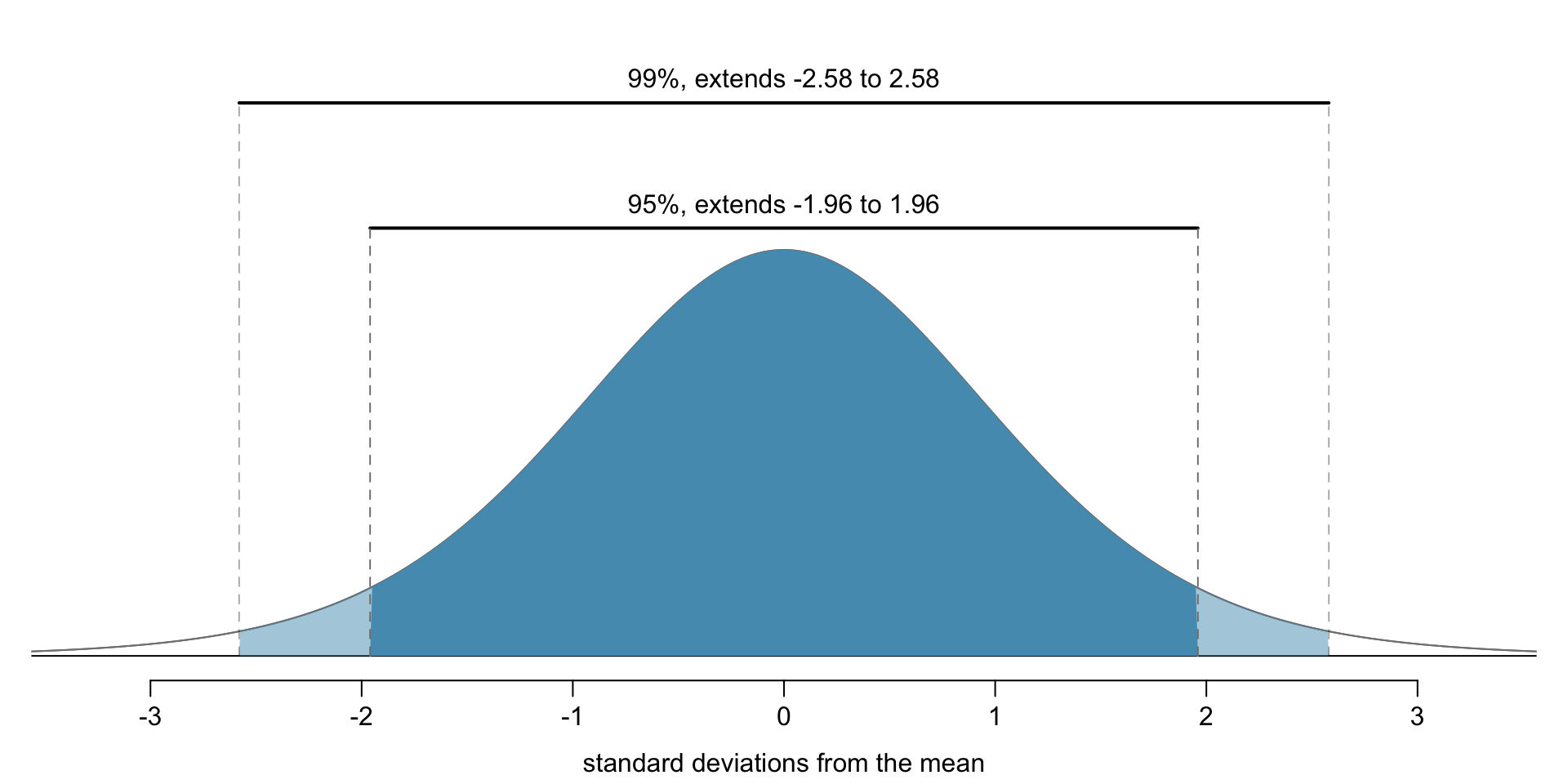
If we want more confidence that our confidence interval contains $p$, the interval should be LARGER to account for greater uncertainty.

The 95% conf. interval takes the form \[\begin{align*} \text{point estimate} \ \pm \ 1.96 \ \times \ SE \end{align*}\]
1.96 corresponds to the 95% confidence level
2.58 corresponds to 99% confidence level
Where do these numbers come from? The normal approximation.

Figure 1: Normal distribution: probability of falling within 2 or 3 standard deviations from the mean.

We can compute these more exactly using qnorm(): quantile function
99% confidence interval corresponds to 0.5% tail on each side. (0.5% + 99% + 0.5% = 100%)
By symmetry, we can just look for the value corresponding to 0.5th percentile.

qnorm(0.005) # for 99%

[1] -2.575829

qnorm(0.025) # for 95%

[1] -1.959964

Hypothesis test for a proportion

We use Z scores to quickly assess how likely/unlikely the sample proportion differs from a hypothesized proportion.

It normalizes the observed difference by the standard error (expected variability in the sample proportion) under the null hypothesis.

\[\begin{align*} Z = \frac{\hat{p} - p_0}{SE(p_0)} = \frac{\hat{p} - p_0}{\sqrt{p_0(1 - p_0)/n}} \end{align*}\]

When null hypothesis is true, and when the samples are independent and we have sufficiently many samples, \[\begin{align*} np_0 \geq 10, \quad n(1-p_0)\geq 10, \end{align*}\] then $Z$ is approximately a standard normal distribution $N(0,1)$.

Payday Loan Hypothesis Test

Example: let’s again consider whether payday loan borrowers support regulation on the loans that require evaluating debt payments. Suppose we have a random sample of 826 borrowers, and 51% said they support regulation.

Is it reasonable to model $\hat p$ w/ a normal distribution?

Independence holds because it’s a random sample; and $np_0 = 413$ and $n(1-p_0)=413$ (we are using the null parameter $p_0=0.5$ here). Thus normal model is reasonable.

What hypothesis should we be testing?

$H_0$: not support for regulation, $p\leq 0.5$.
$H_A$: support for regulation, $p>0.5$.

Under a significance level $\alpha = 0.05$, should we reject $H_0$ given the data?

Let’s first try deciding using Z-score.
$SE(p_0) = \sqrt{\frac{p_0(1-p_0)}n} = \sqrt{\frac{0.5(1-0.5)}{826}} = 0.017$.
Based on the normal model, the test statistic can be computed as the Z score of the point estimate: \[\begin{align*} Z = \frac{\hat{p} - p_0}{SE(p_0)} = \frac{0.51 - 0.5}{0.017} = 0.59 \end{align*}\] $\hat{p}$ within 1 std dev of the mean, so don’t reject $H_0$
Now try p-value (area of shaded region).

normTail(0.5, 0.017, U = 0.51, col = IMSCOL["blue", "full"])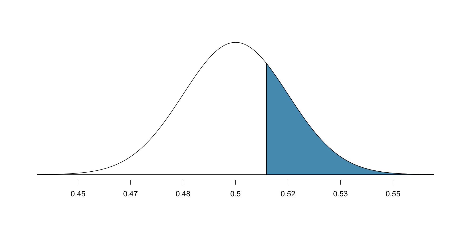

Tail area which represents the p-value is 0.2776.
B/c p-value is larger than 0.05, do not reject $H_0.$

Conclusion: The poll does not provide convincing enough evidence that a majority of payday loan borrowers support loan regulations.