library(tidyverse)
library(openintro)
library(infer)

library(knitr)
library(ggpubr)
library(kableExtra)
library(gghighlight)

library(patchwork)

options(pillar.print_min = 9)  # to avoid annoying scroll behavior
knitr::opts_chunk$set(out.height = "100%")
theme_set(theme_bw())
Inference with mathematical models
STA35B: Statistical Data Science 2
Sampling distributions
A sampling distribution is the distribution of all possible values of a sample statistic from samples of a given sample size from a given population.
- Describes how much sample statistics vary from one sample to another.
- E.g. mean GPA of 7 randomly sampled UC Davis data-science graduates.
Because a sampling distribution describes sample statistics computed from many studies, it cannot be visualized directly from a single dataset.

- Can only be visualized using computational methods / mathematical models.
In previous examples, we ran 10,000 simulations under the null hypothesis \(H_0\).
- Each simulation provided a version of the sample statistic under \(H_0\).
- These 10,000 versions allowed us to estimate the sampling distribution of the sample statistic under \(H_0\), i.e., the null distribution.
- We visualize our estimated null distributions below:
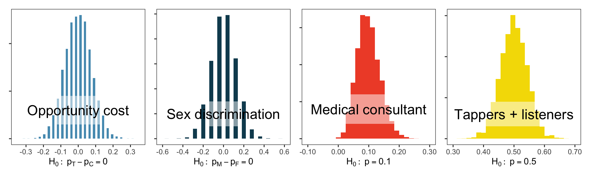
- These distribution shapes look oddly similar to each other…
The central limit theorem and normal distributions
Central limit theorem: With enough independent samples from a population, the sample proportion/mean will increasingly resemble a normal distribution, which is a bell-shaped curve that looks like
- \(\mu\) (Greek letter “mu”) is the distribution mean (a location parameter)
- \(\sigma\) (Greek letter “sigma”) is the distribution “standard deviation” (a scale parameter)
Values of \(\mu\), \(\sigma\) may change from plot to plot, but retains the bell shape. E.g.:
- The sample proportion \(\hat p\) will look like a normal distribution centered at population proportion \(p\) provided that:
- The observations in the sample are independent: samples are truly randomly sampled from a population.
- Sample size is large enough: each class (treatment/control) generally needs \(\geq 10\) observations.
- Same ideas hold for sample mean \(\bar x\): centered at population mean \(\mu\).
Normal distribution model
- Symmetric, unimodal, bell-shaped. Area under curve always integrates to 1.
- Exact values of center / spread can change.
- Mean \(\mu\) shifts from left to right.
- Standard deviation \(\sigma\) squishes or stretches the bell shape.
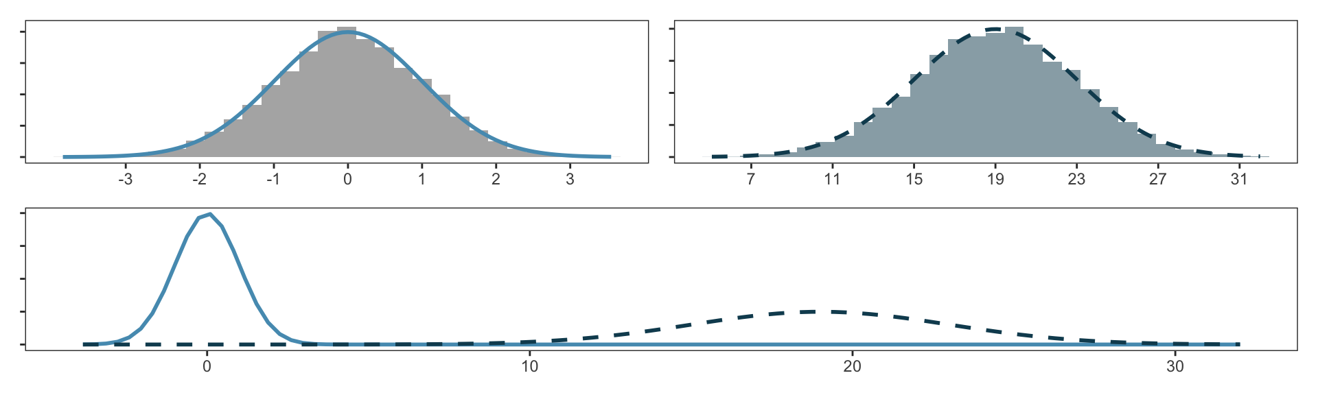
We denote “normal distribution with mean \(k\) and standard deviation \(r\)” as \(N(\mu = k, \sigma = r)\).
- Left curve has \(N(\mu=0, \sigma=1)\); right curve has \(N(\mu=19, \sigma=4)\).
- We call \(N(\mu=0, \sigma=1)\) the standard normal distribution.
Normal probability calculations: percentile and quantile
Ant scored 1800 on SAT. What is the percentile of this score?
openintro::normTail(m = 1500, s = 300, L = 1800, cex.lab=1.5, cex.axis=1.5)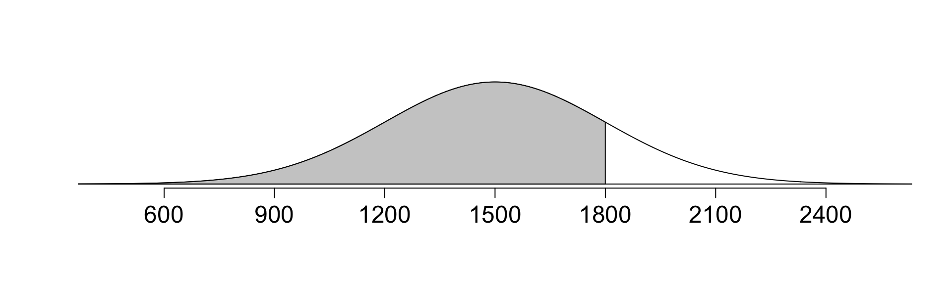
pnorm()provides percentile associated with a cutoff in the normal curve.
pnorm(1800, mean = 1500, sd = 300) # percentile[1] 0.8413447# Can also calculate percentiles as a function of the z-score.
# From previous slide, this corresponds to a z-score of 1.
pnorm(1, mean = 0, sd = 1) # percentile[1] 0.8413447normTail(m = 0, s = 1, L = 0.8413447)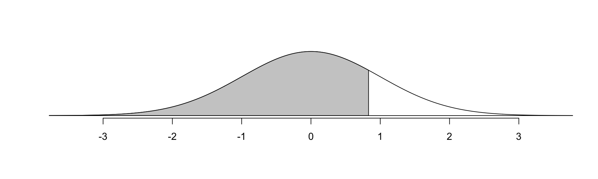
Can also do the reverse: identify the SAT/z-score associated with a percentile.
qnorm(): identifies quantile for given percentage
qnorm(0.8413447, mean = 1500, sd = 300) # SAT score[1] 1800qnorm(0.8413447, mean = 0, sd = 1) # z-score[1] 0.9999998- quantile and percentile are inverse operations:
3 |> pnorm(mean = 0, sd = 1) |> qnorm(mean = 0, sd = 1)[1] 30.99 |> qnorm(mean = 5, sd = 3) |> pnorm(mean = 5, sd = 3)[1] 0.99Normal probability calculations: area
What is the probability that a random SAT taker scores \(\geq 1630\)?
- Recall: normal, mean \(\mu=1500\), s.d. \(\sigma=300\).
- Draw the normal curve and visualize the problem:
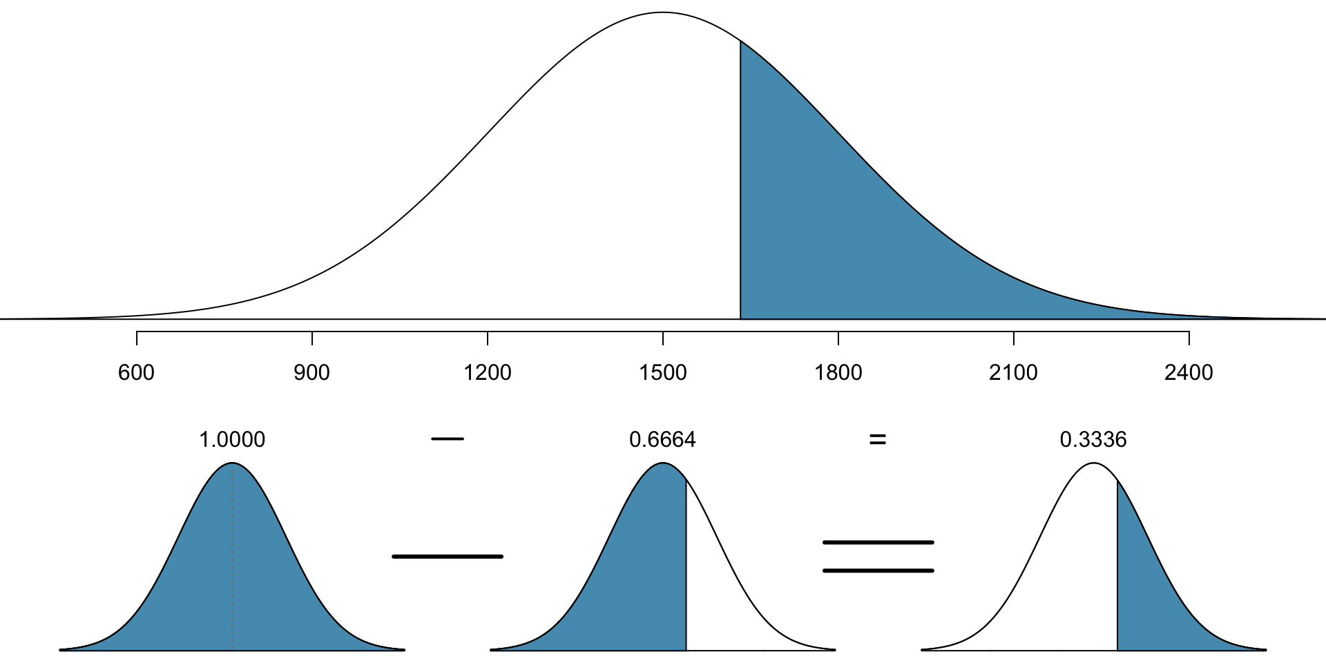
- Calculate z-score of 1630: \[ Z = \frac{x - \mu}{\sigma} = \frac{1630 - 1500}{300} = \frac{130}{300} = 0.433.\]
- Then we want to calculate the percentile:
pnorm(130/300, mean = 0, sd = 1)[1] 0.6676137pnorm(1630, mean = 1500, sd = 300)[1] 0.6676137- Thus the proportion of 0.668 have people with z-score lower than 0.433.
- To compute area above, need to take one minus this (total area = 1)
- Total proportion: \(1-0.668 = 0.332\).
- Probability of scoring at least 1630 is 0.332, or 33.2%.
Ex: SAT
Suppose Dog scored 1400 on SAT. What percentile is this?
- Draw a picture:
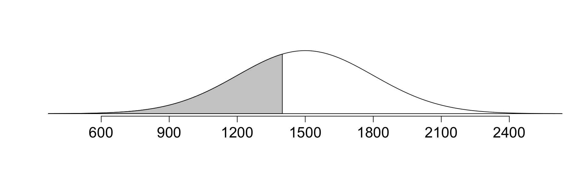
Approach 1: use data directly.
pnorm(1400, mean = 1500, sd = 300)[1] 0.3694413Approach 2: first calculate z-score, then use pnorm() on z-score.
- Calculate z-score: \[ Z = \frac{x - \mu}{\sigma} = \frac{1400 - 1500}{300} = \frac{-100}{300} = -0.333.\]
pnorm(-100/300, mean = 0, sd = 1)[1] 0.3694413Either approach: Dog did better than ~37% of SAT takers.
Ex: Height
Suppose the height of men is approx. normal with avg 70” and sd 3.3”
- If Ewe is 5’7” (67”), Fox is 6’4” (76”), what percentile of men are their heights? Draw a picture and use
pnorm()to calculate the percentage.
normTail(70, 3.3, L = 67, cex.lab=2, cex.axis=2)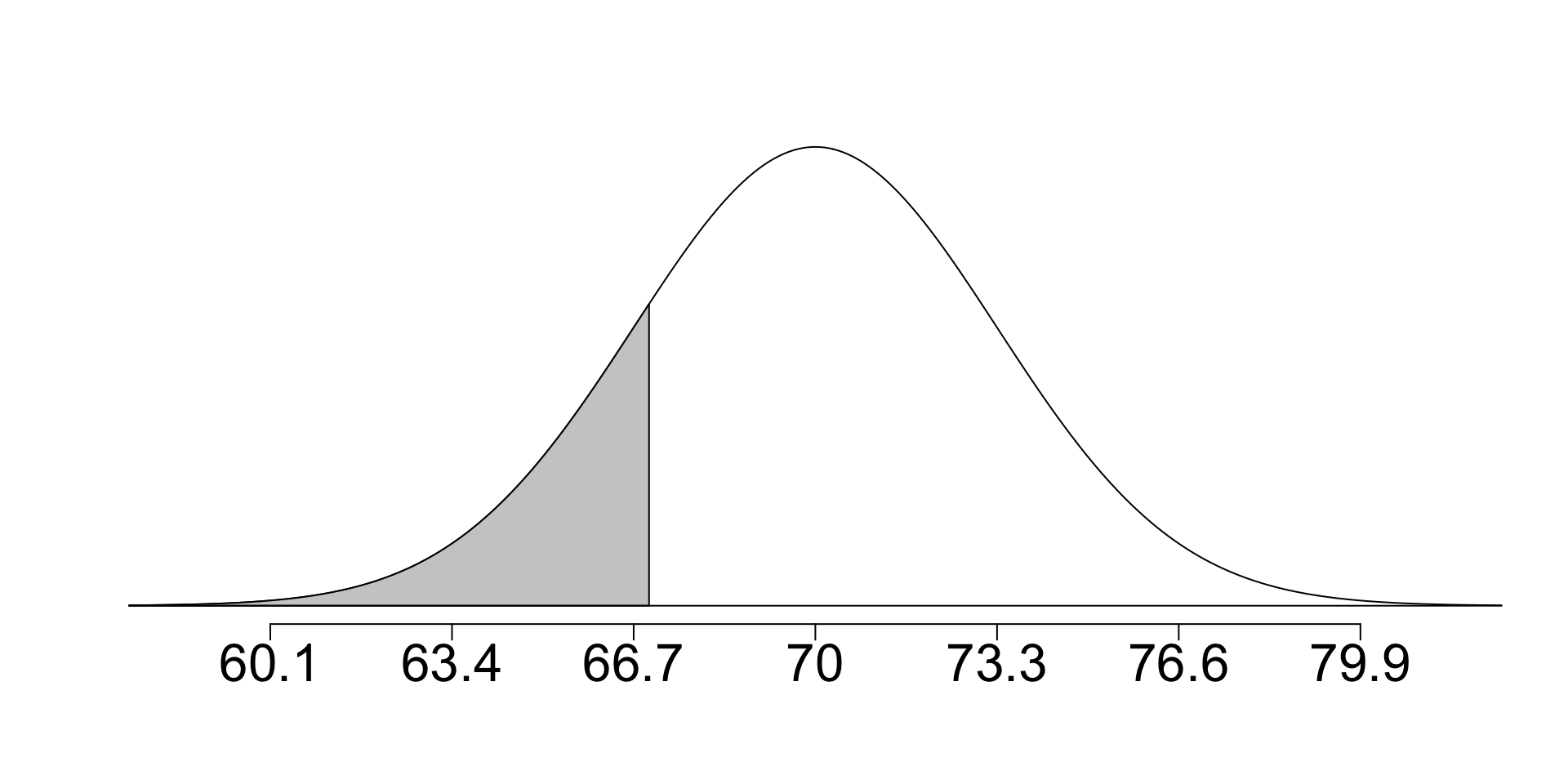
pnorm(67, mean = 70, sd = 3.3)[1] 0.1816511normTail(70, 3.3, L = 76, cex.lab=2, cex.axis=2)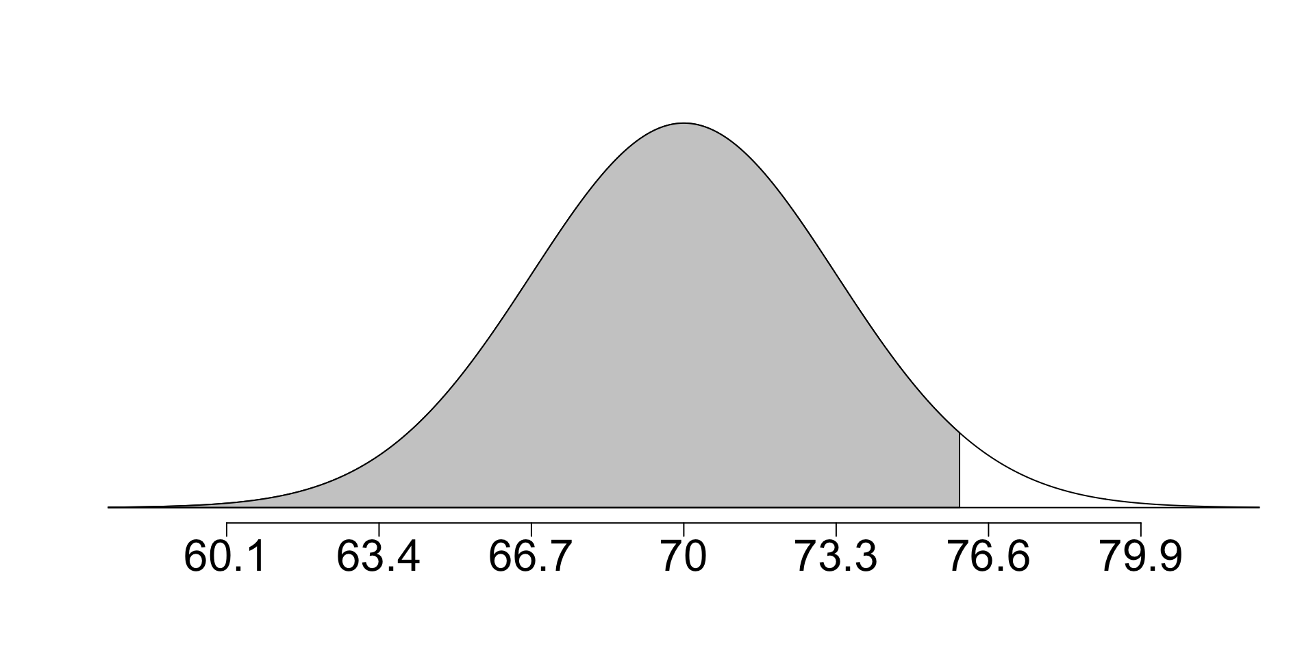
pnorm(76, mean = 70, sd = 3.3)[1] 0.9654818Ex: Height Percentiles
- Let’s now try and calculate what the 40th percentile for height is
- Mean: 70”, s.d.: 3.3”
- Always draw a picture first:
normTail(70, 3.3, L = qnorm(0.4, 70, 3.3), col = IMSCOL["blue", "full"])
text(67, 0.03, "40%\n(0.40)", cex = 1, col = IMSCOL["black", "full"])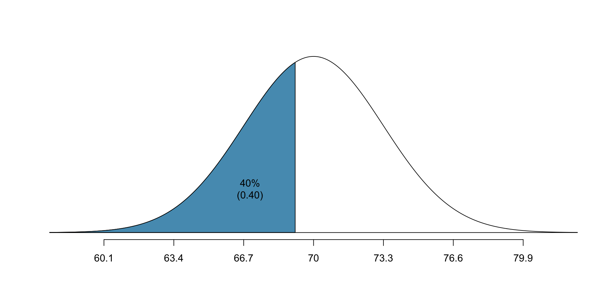
- z-score associated with 40th percentile:
qnorm(0.4, mean = 0, sd = 1)[1] -0.2533471- With z-score, mean, and s.d., we can calculate the height: \[-0.253 = Z = \frac{x-\mu}{\sigma} = \frac{x - 70}{3.3} \] \[ \implies x - 70 = 3.3 \times -0.253 \] \[ \implies x = 70 - 3.3\times 0.253 = 69.18 \]
- 69.18” is approximately 5’9”
Quantifying the variability of statistics
Most statistics we have seen (sample proportion, sample mean, difference in two sample proportions/means) are approximately normal when the data is independent and there are enough samples.
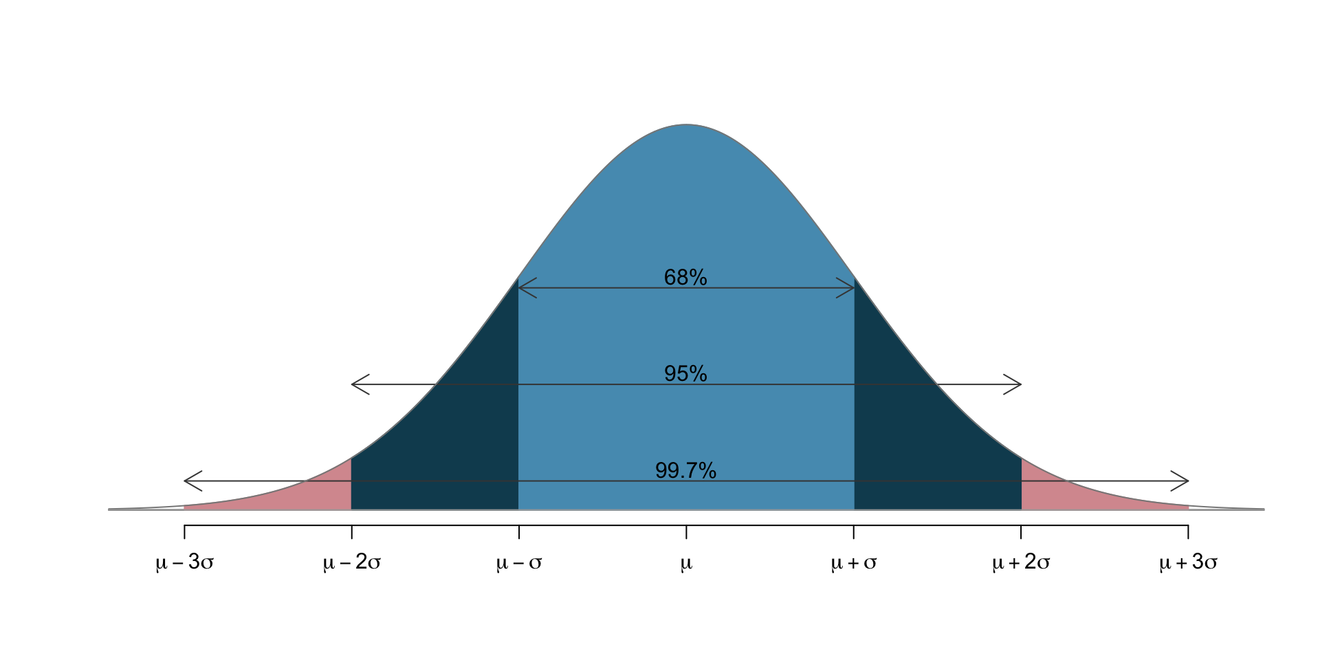
- It is thus very useful to have an intuition for how much variability there is within a few standard deviations of the mean in a normal distribution.
- 68 - 95 - 99.7 rule: pictorally,
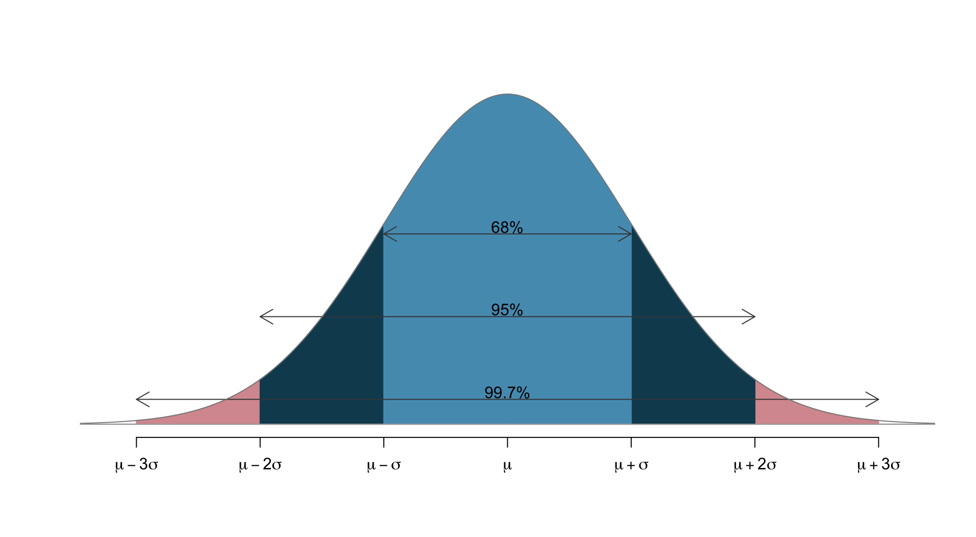
- 68% of the data lies within 1 s.d. of the mean
- 95% lies within 2 s.d.’s
- 99.7% lies within 3 s.d.’s
- Only 0.3% lies more than 3 s.d.’s away from the mean.
- We can confirm this with
pnorm()in R:
pnorm(1, mean=0, sd=1) - pnorm(-1, mean=0, sd=1)[1] 0.6826895pnorm(2, mean=0, sd=1) - pnorm(-2, mean=0, sd=1)[1] 0.9544997pnorm(3, mean=0, sd=1) - pnorm(-3, mean=0, sd=1)[1] 0.99730022 * pnorm(-3, mean=0, sd=1)[1] 0.002699796Opportunity-cost case study
Students are reminded about saving $15 if they don’t buy video game right now.
- We estimated that difference in proportions was 0.20.
- We then used a randomization test to look at the variability in difference of proportions under null hypothesis: difference in proportions does NOT depend on being presented with reminder
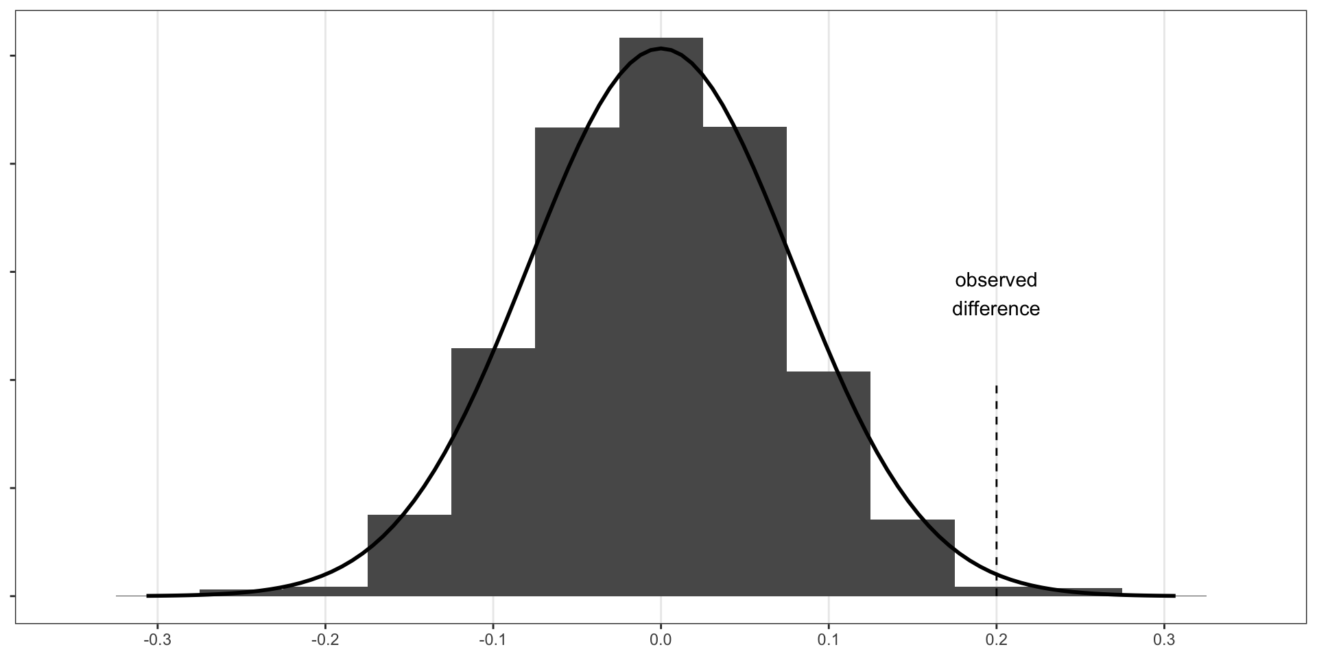
z-score in a hypothesis test is given by substituting the standard error for the standard deviation: \[Z = \frac{\text{observed difference} - \text{null value}}{SE}\]
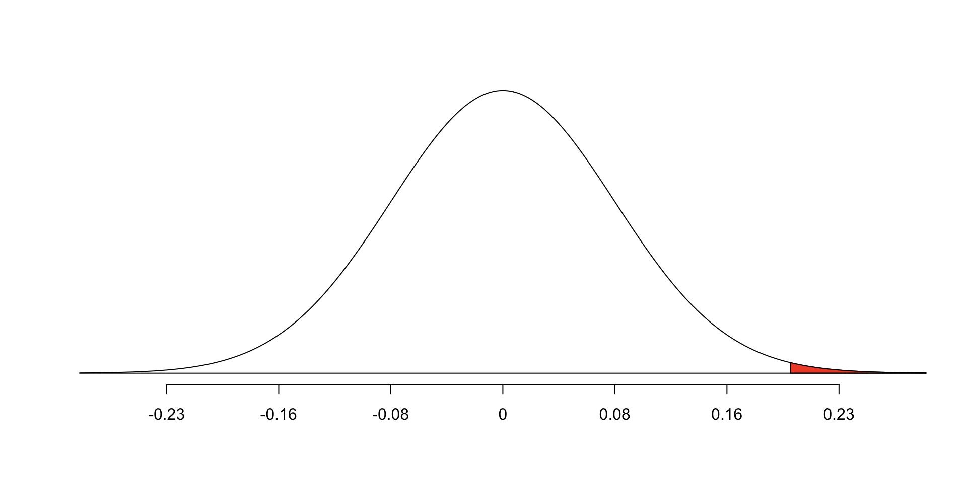
- Here: assume we know the SE is 0.078 (methods to calculate: to come)
\[Z = \frac{0.20 - 0}{0.078} \approx 2.56\]
1 - pnorm(0.2/0.078, mean = 0, sd = 1) # p-value[1] 0.005172149Summary