library(tidyverse)
library(openintro)
library(infer)

library(knitr)
library(ggpubr)
library(kableExtra)
library(gghighlight)

options(pillar.print_min = 9)  # to avoid annoying scroll behavior
knitr::opts_chunk$set(out.height = "100%")
theme_set(theme_bw())Confidence intervals with bootstrapping
STA35B: Statistical Data Science 2
Confidence interval: goal
Our goal here is to understand variability of a statistic (point estimate).
- Randomization tests modeled how the statistic would change if the treatment had been allocated differently.
- Here we instead aim to model how a statistic varies from one sample to another taken from the population.
Bootstrapping: the main idea
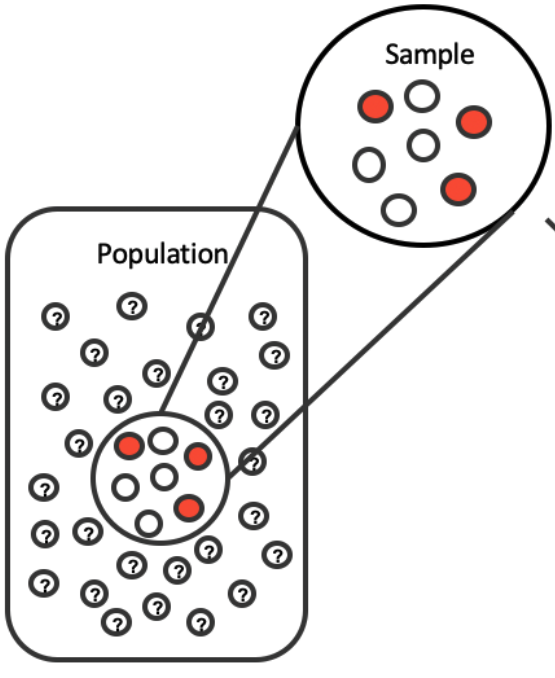
Suppose we have \(x_1, \dots, x_n\) as a random sample from a population.
- If we resample subsets of \(x_1, \dots, x_n\) (with replacement), this “mimics” as if we sample from the true population.
- Medical consultant setting: imagine 3 index cards that say “complication” and 59 that say “no complication”. Put them in big bucket. We shuffle the cards, reach in, record what it says, then put the card back into the bucket, and continue until we have pulled out our desired number of cards.
- This procedure can give us a sense of sample-to-sample randomness.
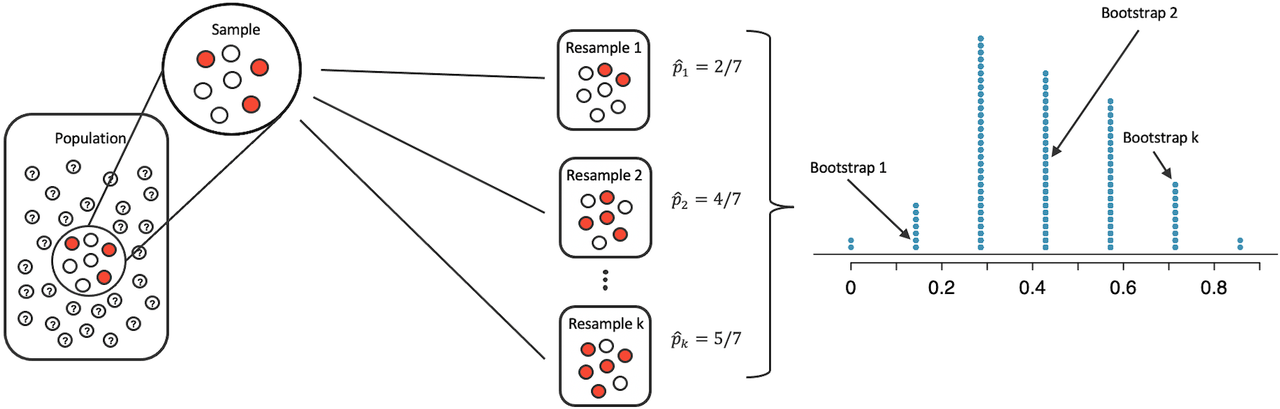
- Each resample is called a bootstrap sample.
- The diagram shows \(k\) bootstrap samples.
- Typically each bootstrap sample has the same number of observations as the original sample (but does not have to be the case).
Medical consultant: bootstrap
- What if we take 10,000 bootstrap samples of the medical consultant data?
- Original data had 62 observations, 3 complications; \(\hat p = 3/62 \approx 0.048\).
prop_obs <- 3 / 62
bsprop <- rbinom(10000, size = 62, prob = prop_obs) / 62
bsprop_025_975 <- quantile(bsprop, c(0.025, 0.975))
bsprop_025_975
2.5% 97.5%
0.0000000 0.1129032 tibble(bsprop) |>
ggplot(aes(x = bsprop)) +
geom_histogram(binwidth = 0.004) +
gghighlight(bsprop <= bsprop_025_975[1] | bsprop >= bsprop_025_975[2]) +
annotate("segment",
x = bsprop_025_975[1], y = 0,
xend = bsprop_025_975[1], yend = 900,
linetype = "dashed"
) +
annotate("segment",
x = bsprop_025_975[2], y = 0,
xend = bsprop_025_975[2], yend = 900,
linetype = "dashed"
) +
annotate("text", x = bsprop_025_975[1], y = 1200,
label = glue::glue("2.5th\npercentile\n({bsprop_025_975[1]})")) +
annotate("text", x = bsprop_025_975[2], y = 1200, ,
label = glue::glue("97.5th\npercentile\n({bsprop_025_975[2]})")) +
labs(
x = "Bootstrapped proportion of surgical complications",
title = "10,000 bootstrapped proportions"
)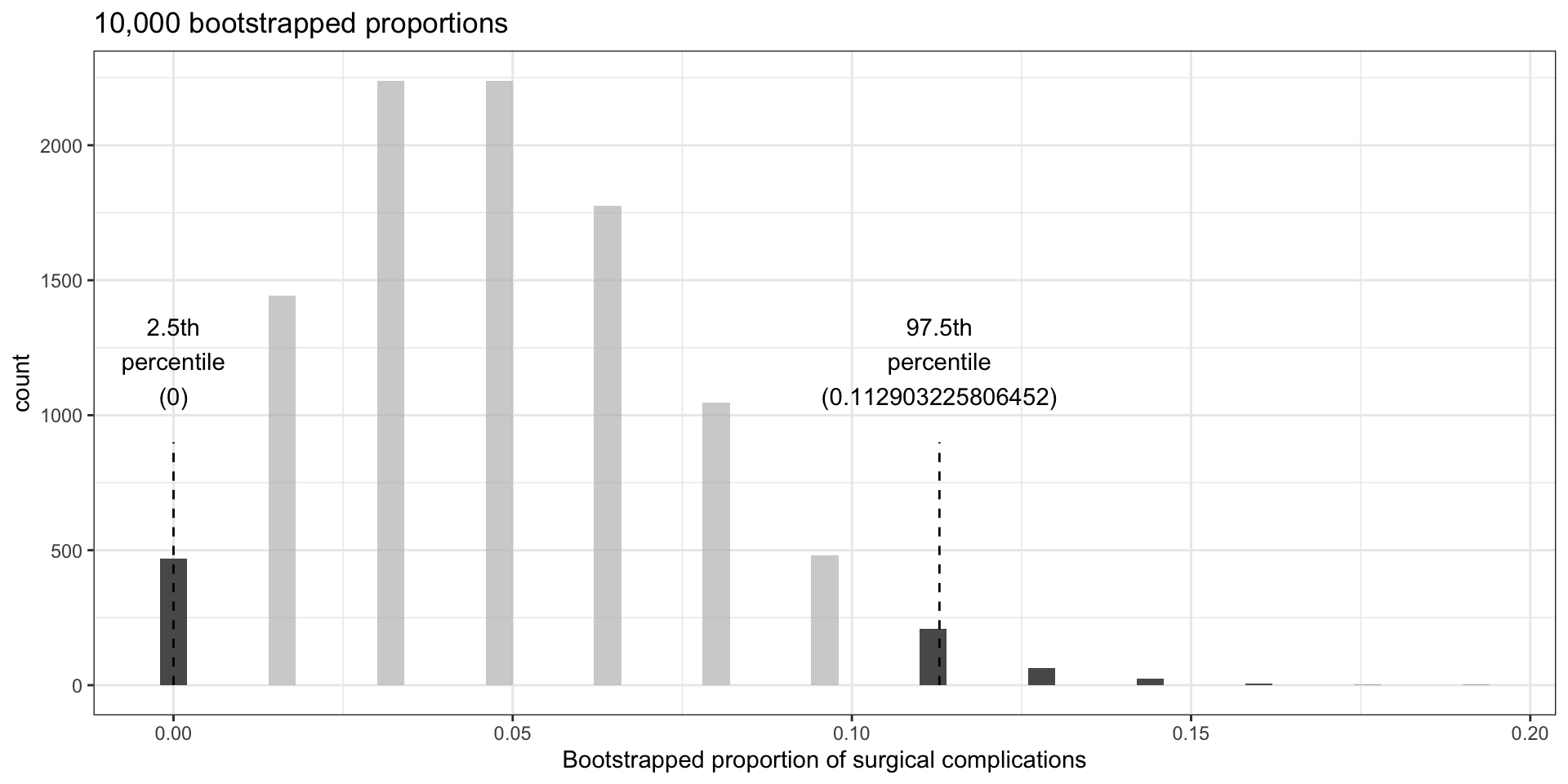
- The 2.5% percentile is at 0; the 97.5th percentile at 0.113.
- Hence we are confident that in the population, the true probability of a complication from the medical consultant is between 0% and 11.3%.
- We were asked to compare this to the national rate of 10%.
- Our interval \((0\%,11.3\%)\) includes 10%, so cannot say that the consultant’s work was associated with a lower risk of complications – could be by chance.
- Even if the interval excluded 10%, we could not make a claim about causality.
Tappers and listeners: bootstrap
We can use bootstrapping as before: imagine we have a jar with 120 marbles, 3 are green (guessed correctly) and 117 are red (could not guess the song).
prop_obs <- 3 / 120
bsprop <- rbinom(10000, size = 120, prob = prop_obs) / 120
bsprop_025_975 = quantile(bsprop, c(0.025, 0.975))
bsprop_025_975
2.5% 97.5%
0.00000000 0.05833333 tibble(bsprop) |>
ggplot(aes(x = bsprop)) +
geom_histogram(binwidth = 0.003) +
gghighlight(bsprop <= bsprop_025_975[1] | bsprop >= bsprop_025_975[2]) +
annotate("segment",
x = bsprop_025_975[1], y = 0,
xend = bsprop_025_975[1], yend = 900,
linetype = "dashed"
) +
annotate("segment",
x = bsprop_025_975[2], y = 0,
xend = bsprop_025_975[2], yend = 900,
linetype = "dashed"
) +
annotate("text", x = bsprop_025_975[1], y = 1200,
label = glue::glue("2.5th\npercentile\n({bsprop_025_975[1]})")) +
annotate("text", x = bsprop_025_975[2], y = 1200, ,
label = glue::glue("97.5th\npercentile\n({bsprop_025_975[2]})")) +
labs(
x = "Bootstrapped proportion of listeners who guessed correctly",
y = "Count",
title = "10,000 bootstrapped proportions"
)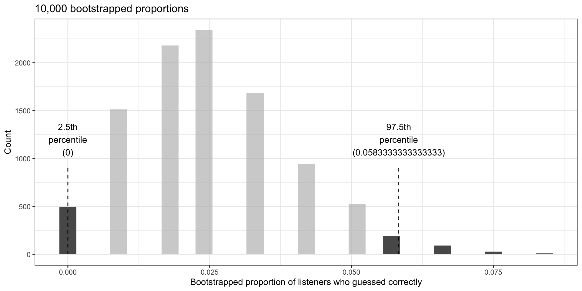
- Expect between 0-5.83% are able to guess tapper’s tune
Youtube videos
Want to estimate proportion of YouTube videos taking place outdoors
- We sample 128 videos and find 37 take place outdoors.
- Want to estimate proportion of all YouTube videos which take place outside.
- What is the relevant statistic and parameter for this problem?
- Statistic: sample proportion \(\hat p = 37/128 \approx 0.289\);
- Parameter: population proportion (\(p\); unknown).
- Let’s construct a bootstrap confidence interval:
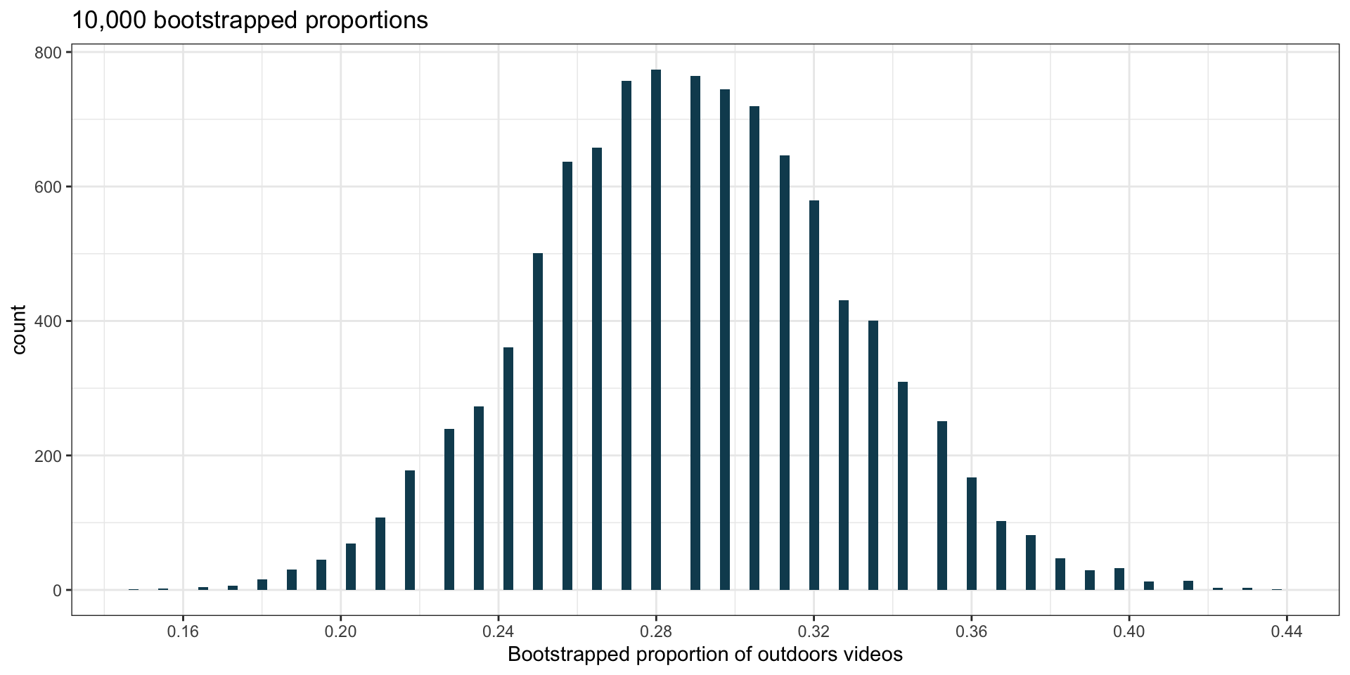
- If we want to be 90% confident that between \(a\)% and \(b\)% of YouTube videos that take place outdoors, how should we find \(a\) and \(b\)?
- We want 5% of values to be below \(a\), and 5% of values to be above \(b\).
- The interval should be centered at \(\hat p \approx 0.289\) (so, \(\hat p = (a + b)/2\)).
- From the graph, we see that \(a\approx 0.22\) and \(b\approx 0.35\) is correct.