Hypothesis testing with randomization

STA35B: Statistical Data Science 2

Akira Horiguchi

Plan for remainder of quarter

Part IV: Foundations of inference (next few decks)

Statistical inference: making conclusions about a population using information in a sample. Different ways to quantify variability seen from dataset to dataset:

  1. Ch 11: randomization which involves repeatedly permuting observations to represent scenarios in which there is no association between two variables of interest. [this slide deck]
  2. Ch 12: bootstrapping which involves repeatedly sampling (with replacement) from the observed data in order to produce many samples which are similar to, but different from, the original data.
  3. Ch 13: Central Limit Theorem which is a theoretical approximation to the variability in data seen through randomization and bootstrapping.

There is almost never a single “correct” approach, and often these methods give similar results.

Part V: Statistical inference

Inference for [scenario]

  1. Randomization test for [scenario].
  2. Bootstrapping confidence interval for [scenario].
  3. Mathematical model(s) for [scenario].

Apply Part IV (tools) to Part V (scenarios)

Statistical inference

Based on Ch 11 of IMS

library(tidyverse)
library(openintro)
library(infer)

library(knitr)
library(ggpubr)
library(kableExtra)
library(gghighlight)

options(pillar.print_min = 9)  # to avoid annoying scroll behavior
knitr::opts_chunk$set(out.height = "100%")
theme_set(theme_bw())

Statistical inference

Statistical inference is concerned with understanding and quantifying uncertainty in parameter estimates.

  • Learn about a population of interest.
  • Often infeasible to collect data on the entire population.
  • We can collect data on a sample of the population to answer a research question about the population.
Examples Sample Population
Polls voters who were polled all voters
Clinical trials a study’s subjects all who have a particular disease
  • We can then learn/infer about the sample, but will those takeaways generalize to the population?

How representative of the population is the data?

  • Consider two datasets from the same population using the same (randomized) methods.
  • These two datasets will typically not be identical; this is due to randomness.
  • Not easy to quantify the variability in the data.
    • i.e., it is not trivial to answer the question “how different is one dataset from another?”
  • Studying randomness of this form is a key focus of statistics.

Why Inference?

The goal of inference is to quantify how likely certain outcomes are due to random chance vs. due to real differences.

  • Think through what would happen if we repeatedly took different surveys of people’s opinions on support for some policy.
  • There will be some natural sample-to-sample variation, but if there is a big difference in support for vs. against the policy, this randomness will be drowned out by the true difference in the population preference.
  • The coming lectures will discuss the hypothesis testing framework: allows for formally evaluating claims about populations.

Let’s look at two motivating examples.

Notation:

  • \(p\) to denote population proportion
    • e.g. proportion of population supporting some policy
  • \(\hat p\) to denote sample proportion
    • e.g. a survey of 1,000 people on whether they support a policy

The “hat” notation is used to denote a statistic computed from a sample, and the non-hat version is used to denote the corresponding parameter in the population.

Example 1: Sex Discrimination Study

Question and data collection

Are female employees discriminated against in promotion decisions made by male managers?

Study (1970s)

  • 48 male bank supervisors were asked to assume the role of the personnel director of a bank.
  • Each supervisor was given a personnel file to judge whether the person should be promoted to a branch manager position.
  • The files given to the supervisor were identical, except that half of the files indicated the candidate identified as male and the other half indicated the candidate identified as female.
  • These files were randomly assigned to the bank managers.

Data

sex_discrimination
# A tibble: 48 × 2
  sex   decision
  <fct> <fct>   
1 male  promoted
2 male  promoted
3 male  promoted
4 male  promoted
5 male  promoted
6 male  promoted
7 male  promoted
8 male  promoted
9 male  promoted
# ℹ 39 more rows
table(sex_discrimination)
        decision
sex      promoted not promoted
  male         21            3
  female       14           10
table(sex_discrimination) |> addmargins()
        decision
sex      promoted not promoted Sum
  male         21            3  24
  female       14           10  24
  Sum          35           13  48
table(sex_discrimination) |> addmargins() |> kable()
promoted not promoted Sum
male 21 3 24
female 14 10 24
Sum 35 13 48
  • 24 male candidates, 24 female candidates.
  • Proportion of promoted males is \(\hat{p}_M^{obs} = 21 / 24\).
  • Proportion of promoted females is \(\hat{p}_F^{obs} = 14 / 24\).
  • Difference of proportions is \(\hat{p}_M^{obs} - \hat{p}_F^{obs} = 7/24 \approx 0.292\).

\(\hat{p}_M^{obs} - \hat{p}_F^{obs}\) is a point estimate of the population difference \(p_M - p_F\).

Hypotheses

We can formulate two competing claims (hypotheses) about the relationship between sex and promotions:

  • \(H_0\), Null: sex and decision are independent. Observed differences in proportions promoted are due to natural variability.
    • E.g.: \(p_M = p_F\). Equivalent to \(p_M - p_F = 0\).
  • \(H_A\), Alternative: sex and decision are dependent. Observed differences in proportions are due to dependence between the two variables.
    • E.g.: \(p_M > p_F\). Equivalent to \(p_M - p_F > 0\).

Variability of the statistic under the null hypothesis

We can use a permutation test to examine whether \(H_0\) is true.

  • Suppose the bankers’ decisions were independent of the sex of the candidate.
  • Then if we randomly shuffled all of the labels of “male” and “female”, any difference in promotion rates would be due to chance.
  • Let’s now shuffle the labels of male / female among the 48 study subjects.
    • How to code a random shuffle? sample(x) permutes the values in a vector x.
set.seed(37)  # to enable reproducibility of "random" outcomes
sex_disc_rand_1 <- tibble(
  sex = sample(sex_discrimination$sex),  # shuffled version of `sex` column in `sex_discrimination`
  decision = sex_discrimination$decision
)
sex_disc_rand_1
# A tibble: 48 × 2
  sex    decision
  <fct>  <fct>   
1 female promoted
2 male   promoted
3 male   promoted
4 female promoted
5 female promoted
6 female promoted
7 female promoted
8 male   promoted
9 male   promoted
# ℹ 39 more rows
sex_disc_rand_1 |> table() |> addmargins() |> kable()
Table 1: Simulation results, where the difference in promotion rates between male and female is purely due to random chance.
promoted not promoted Sum
male 16 8 24
female 19 5 24
Sum 35 13 48

We can compute the point estimate \(\hat{p}_M^{(1)} - \hat{p}_F^{(1)}\) for this shuffle #1.

Distribution of the statistic under the null hypothesis

We can perform multiple shuffles to get a sense of the distribution of the promotion-rate differences under the null hypothesis \(H_0\).

  • In theory, one could do all \(48!\) possible shuffles to get the exact distribution of promotion-rate differences under \(H_0\).
  • We will instead randomly draw 10,000 of these \(48!\) possible shuffles to get an approximate distribution of promotion-rate differences under \(H_0\):
    • For \(j=1,2,3,\ldots,10000\):
      • Shuffle the data; call it the \(j\)th shuffle.
      • Compute the difference \(\hat{p}_M^{(j)} - \hat{p}_F^{(j)}\) for this shuffle \(j\).
  • (We’ll assume that this distribution of 10,000 differences will closely approximate the exact distribution of all \(48!\) differences.)
  • We could code this procedure ourselves, but let’s use openintro functions:
set.seed(37)
shuff_df <- sex_discrimination |>
  specify(decision ~ sex, success = "promoted") |>
  hypothesize(null = "independence") |>
  generate(reps = 10000, type = "permute") |>
  calculate(stat = "diff in props", order = c("male", "female"))
shuff_df
Response: decision (factor)
Explanatory: sex (factor)
Null Hypothesis: indepe...
# A tibble: 10,000 × 2
  replicate    stat
      <int>   <dbl>
1         1 -0.0417
2         2  0.0417
3         3 -0.125 
4         4 -0.208 
5         5  0.0417
6         6 -0.125 
7         7  0.0417
8         8 -0.292 
9         9  0.125 
# ℹ 9,991 more rows
  • Visualize the distribution of these 10,000 difference (stat) values.
p_shuff <- shuff_df |> 
  ggplot(aes(x = stat)) +
  geom_histogram(binwidth = 0.01) +  # set `binwidth = 0.01` to emphasize that there are only a few unique values
  scale_x_continuous(breaks=seq(-1, 1, by=0.2)) +
  scale_y_continuous(sec.axis = dup_axis(),  # Mirrors the left axis on the right + 
                     breaks=seq(0, 10000, by=400)) + 
  labs(
    title = "10,000 differences in randomized proportions",
    x = "Differences in promotion rates (male - female) across 10000 shuffles"
  )
p_shuff
A histogram plot of proportion differences from 10000 simulations produced under the null hypothesis, $H_0,$ where the simulated sex and decision are independent.
Figure 1: A histogram plot of proportion differences from 10000 shuffles produced under the null hypothesis, \(H_0,\) where the simulated sex and decision are independent.
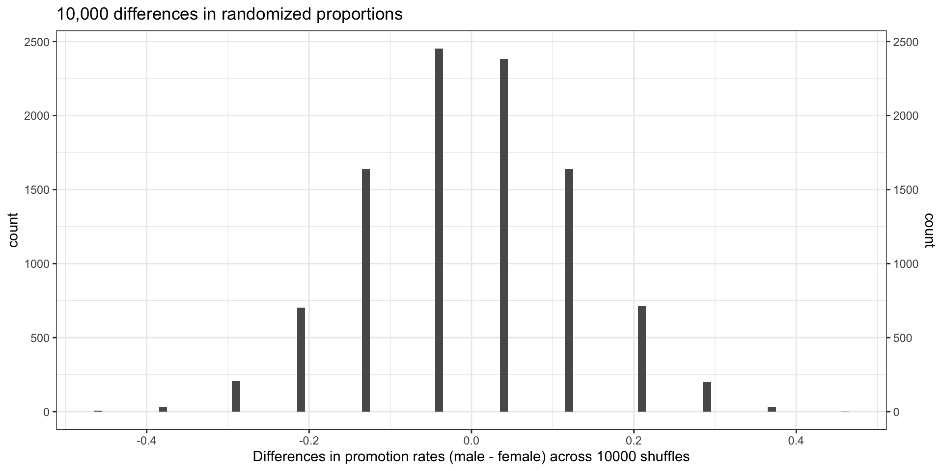
  • (Why are there so few unique difference values?)

How does the observed value compare?

How many of the \(\hat{p}_M^{(j)} - \hat{p}_F^{(j)}\) were \(\geq\) the observed \(\hat{p}_M^{obs} - \hat{p}_F^{obs} = \frac{7}{24}\)?

obs_prop_diff <- 21/24 - 14/24  # difference of proportions in the "true" observed data
n_at_least_as_large <- sum(shuff_df$stat >= obs_prop_diff)
n_at_least_as_large
[1] 230

Visualize how the observed value compares to the distribution under \(H_0\).

p_shuff + 
  geom_vline(xintercept=obs_prop_diff, linetype='dashed') +  # dashed vertical line
  gghighlight(stat >= obs_prop_diff) 

Same histogram plot, but now highlighting which shuffles produce a proportion difference is at least as large as the observed proportion difference.

Same histogram plot, but now highlighting which shuffles produce a proportion difference is at least as large as the observed proportion difference.
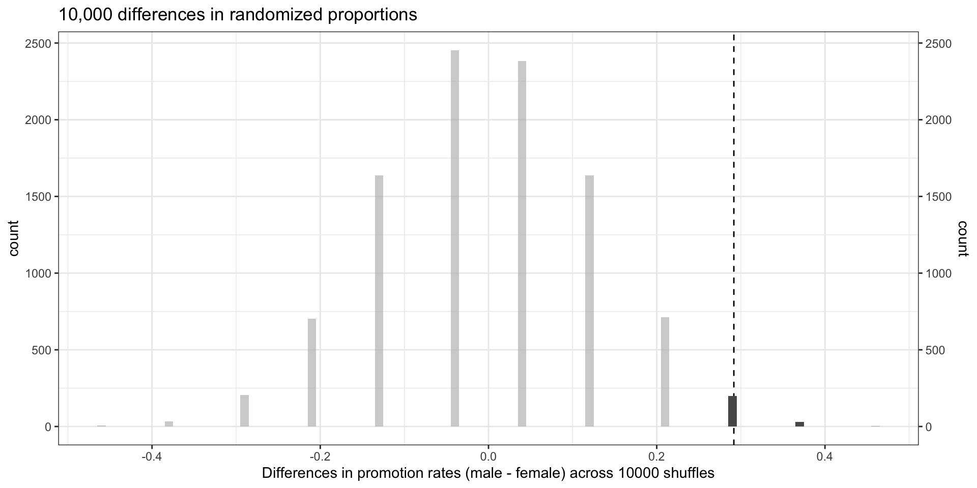
  • Only 230 of the 10,000 shuffles had \(\hat{p}_M^{(j)} - \hat{p}_F^{(j)} \geq \frac{7}{24}\).
  • Hence the observed difference \(\frac{7}{24} \approx 0.292\) is unlikely to have occurred simply by chance under \(H_0\).
  • Suggests that hiring and sex were not independent.

Hypothesis testing

Earlier we described a hypothesis test:

  • Null hypothesis: belief that things could have happened due to chance
  • Alternative hypothesis: there is some relationship between variables

Way to think about it: trial by jury

  • Null hypothesis: not guilty.
  • Alternative hypothesis: guilty.
  • We might reject the null in favor of the alternative if there is discernible evidence in favor of this claim.
  • Failure to reject the null does not mean null is true, just that we don’t have enough evidence to reject the null.

p-values and statistical discernibility

A \(p\)-value represents the probability that, if the null hypothesis is true, we would obtain data that is at least as extreme as the result actually observed.

  • When the \(p\)-value is smaller than a threshold \(\alpha\) (called a discernibility level), then we say that the results are statistically discernible at level \(\alpha\), and we reject the null hypothesis in favor of the alternative.
    • Often use \(\alpha=0.1\) or \(\alpha=0.05\) or \(\alpha=0.01\), but depends on context.
  • Example 1: in sex-discrimination study,
    • Only 230 of 10,000 had a larger value, so the \(p\)-value is \(\approx\) 0.023.
    • There is discernible evidence at level \(\alpha=0.05\) to reject \(H_0\).

Discernibility vs significance

  • You may have heard the phrase “statistically significant”.
    • “Significant” can be misleading; in everyday language “significant” would indicate that a difference is large or meaningful.
    • Recent push toward switching to “discernible”.

Interpreting discernible evidence

How to interpret statistically discernible evidence?

  • How the data was produced/collected? By experiment or by observation?

Example 1: the sex-discrimination study is an experiment: subjects were randomly assigned a “male” file or a “female” file (remember, all the files were actually identical in content).

  • Because this is an experiment, the results can be used to evaluate a causal relationship between the sex of a candidate and the promotion decision.
  • Conclusion: “There is statistically discernible evidence (\(p\)-value \(\approx\) 0.023) that female employees are discriminated against in promotion decisions made by male managers.

But suppose instead that the data had been observational.

  • Then no claim that sex caused difference in hiring outcomes.
  • Correlation does not imply causation!
  • There could be confounding variables: e.g., age, experience, pedigree.
  • Always ask ourselves: “Of what population is this a random sample?”
  • (Weaker) conclusion: “There is statistically discernible evidence (\(p\)-value \(\approx\) 0.023) that female employees in this population are promoted less often than male employees in this population.

Randomization tests summary

  • Frame research question in terms of hypotheses.
    • Null hypothesis \(H_0\): skeptical of any relationship between variables.
    • Alternative hypothesis \(H_A\): posits a relationship between variables.
  • Collect data.
  • Model randomness that would occur if null hypothesis were true.
    • Randomize treatments.
  • Analyze data and identify \(p\)-value.
  • Form conclusion about hypotheses using \(p\)-value.

Example 2: Student Savings

Question and data collection

Let’s consider a study where we ask whether telling a college student that they can save money for later purchases will make them spend less now.

  • \(H_0\): reminding students that they can save money for later purchases will not have any impact on students’ spending decisions.
  • \(H_A\): reminding students that they can save money for later purchases will reduce the chance they will continue with a purchase.

“Imagine that you have been saving some extra money on the side to make some purchases…”

Half of the 150 students were randomized into a control group and given the following options:

  1. Buy this entertaining video.
  2. Not buy this entertaining video.

Remaining 75 students were placed in treatment group, they saw:

  1. Buy this entertaining video.
  2. Not buy this entertaining video. Keep the $14.99 for other purchases.

Data

Dataset: opportunity_cost in openintro

opportunity_cost
# A tibble: 150 × 2
  group   decision 
  <fct>   <fct>    
1 control buy video
2 control buy video
3 control buy video
4 control buy video
5 control buy video
6 control buy video
7 control buy video
8 control buy video
9 control buy video
# ℹ 141 more rows
opportunity_cost |> table() |> addmargins() |> kable()
buy video not buy video Sum
control 56 19 75
treatment 41 34 75
Sum 97 53 150

\[\hat{p}_{T} - \hat{p}_{C} = \frac{34}{75} - \frac{19}{75} = \frac{15}{75} = 0.2\]

  • Under treatment, 20 percentage points higher choose to not buy the video.

  • How much variability would one expect if the treatment had no effect?

  • We can do the same type of analysis from the previous example.

How likely is the observed difference under the null hypothesis?

  • Let’s first look at a single shuffle
opportunity_cost_rand_1 <- tibble(
  group = c(rep("control", 75), rep("treatment", 75)),
  decision = c(
    rep("buy video", 46), rep("not buy video", 29),
    rep("buy video", 51), rep("not buy video", 24)
  )
) |>
  mutate(
    group = as.factor(group),
    decision = as.factor(decision)
  )

opportunity_cost_rand_1 |>
  count(group, decision) |>
  pivot_wider(names_from = decision, values_from = n) |>
  janitor::adorn_totals(where = c("col", "row")) |>
  kbl(linesep = "", booktabs = TRUE) |>
  kable_styling(
    bootstrap_options = c("striped", "condensed"),
    full_width = FALSE
  ) |>
  add_header_above(c(" " = 1, "decision" = 2, " " = 1)) |>
  column_spec(1:4, width = "7em")
decision
group buy video not buy video Total
control 46 29 75
treatment 51 24 75
Total 97 53 150

We can compute a difference that occurred from the first shuffle of the data:

\[\hat{p}_{T}^{(1)} - \hat{p}_{C}^{(1)} = \frac{24}{75} - \frac{29}{75} = - \frac{5}{75} \approx - 0.067\]

  • Compare this to the 20 percentage points (0.2) that we saw before.

Shuffing distribution

Now repeat 10000 times; plot results

set.seed(25)
opportunity_cost_rand_dist <- opportunity_cost |>
  specify(decision ~ group, success = "not buy video") |>
  hypothesize(null = "independence") |>
  generate(reps = 10000, type = "permute") |>
  calculate(stat = "diff in props", order = c("treatment", "control")) |>
  mutate(stat = round(stat, 3))
opportunity_cost_rand_dist
Response: decision (factor)
Explanatory: group (factor)
Null Hypothesis: inde...
# A tibble: 10,000 × 2
  replicate   stat
      <int>  <dbl>
1         1  0.04 
2         2  0.12 
3         3 -0.013
4         4 -0.12 
5         5  0.04 
6         6 -0.067
7         7  0.04 
8         8 -0.04 
9         9  0.04 
# ℹ 9,991 more rows
opportunity_cost_rand_dist |> 
  ggplot(aes(x = stat)) +
  geom_histogram(binwidth = 0.005) +
  geom_vline(xintercept = 0.20, linetype='dashed') +
  gghighlight(stat >= 0.20) +
  scale_y_continuous(sec.axis = dup_axis()) +  # Mirrors the left axis on the right
  labs(
    title = "10,000 differences in randomized proportions",
    x = "Difference in randomized proportions of students who\ndo not buy the video (treatment - control)",
    y = "Count\n(Number of simulated scenarios)"
  )
Figure 2: A histogram of 10,000 chance differences produced under the null hypothesis.
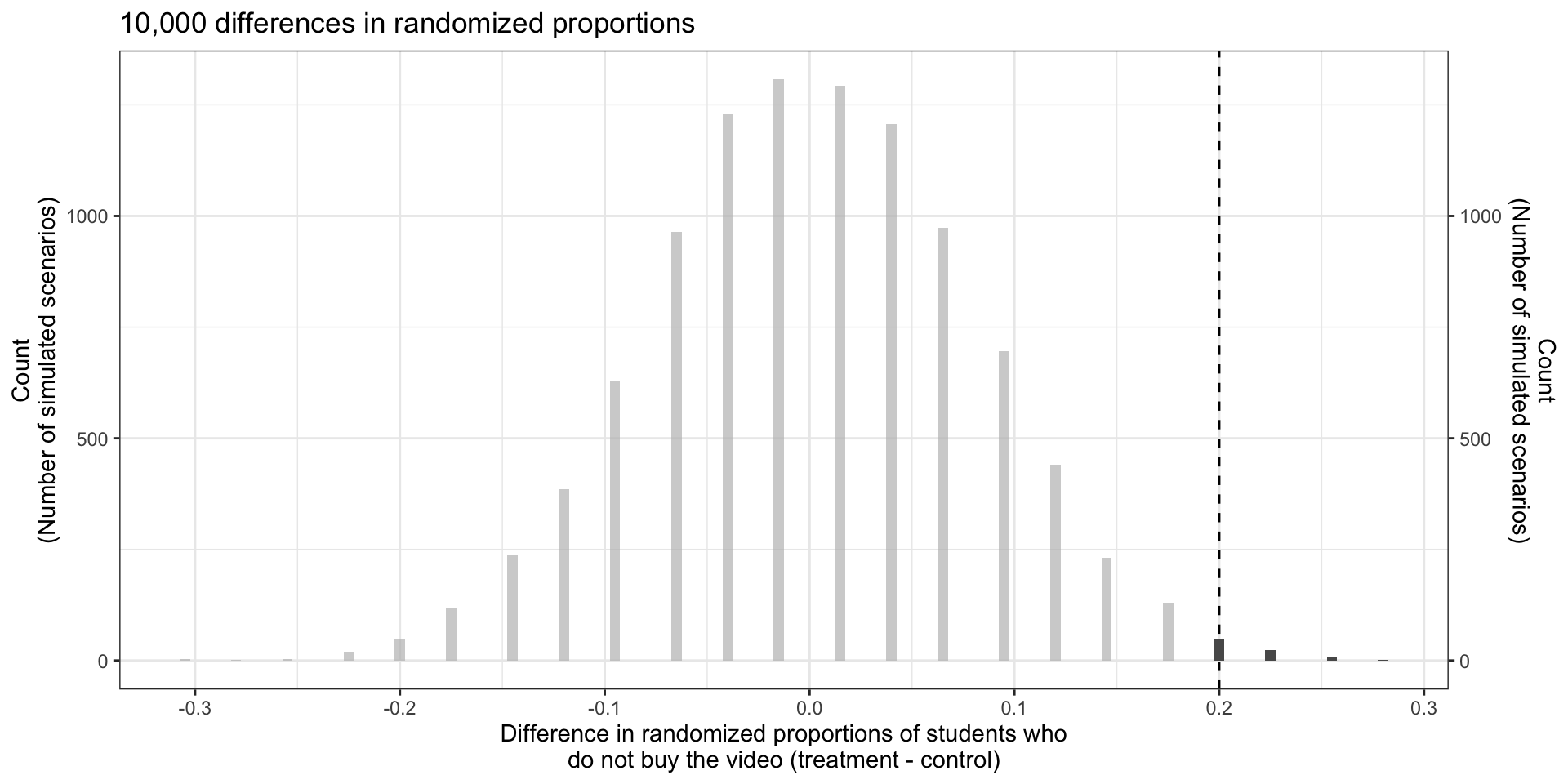
  • Only 83 of the 10,000 shuffles had proportion difference \(\geq 0.20\). Then the \(p\)-value is \(\approx\) 0.0083.
  • Statistically discernible at level \(\alpha=0.01\), i.e., there is discernible evidence at level \(\alpha=0.01\) to reject \(H_0\).
  • “The data provide statistically discernible evidence that US college students were actually influenced by the reminder.”