13: linear regression with multiple predictors

STA35B: Statistical Data Science 2

Akira Horiguchi

Linear regression

library(ggplot2)
library(tidyverse)
library(unvotes)
library(knitr)
library(scales)
library(ggpubr)  # for statcor()
library(broom)  # for tidy()
library(openintro)
library(patchwork)

Linear regression with multiple predictors

Multiple regression extends single predictor regression by allowing multiple predictors $x_1, x_2, x_3, \ldots$

\[y = b_0 + b_1 x_1 + b_2 x_2 + \cdots\]

Data: loans_full_schema data with tidying

loans <- loans_full_schema |>
  mutate(
    credit_util = total_credit_utilized / total_credit_limit,
    bankruptcy  = as.factor(if_else(public_record_bankrupt == 0, 0, 1)),
    verified_income = droplevels(verified_income)
    ) |>
  rename(credit_checks = inquiries_last_12m) |>
  select(interest_rate, verified_income, debt_to_income, credit_util, bankruptcy, term, credit_checks, issue_month)

Linear regression with multiple predictors

loans |>
  slice_head(n = 5) |>
  kableExtra::kbl(linesep = "", booktabs = TRUE, align = "rlrrrr") |>
  kableExtra::kable_styling(
    bootstrap_options = c("striped", "condensed"),
    latex_options = c("striped", "scale_down", "hold_position"),
    full_width = FALSE
  )

interest_rate	verified_income	debt_to_income	credit_util	bankruptcy	term	credit_checks	issue_month
14.07	Verified	18.01	0.5475952	0	60	6	Mar-2018
12.61	Not Verified	5.04	0.1500347	1	36	1	Feb-2018
17.09	Source Verified	21.15	0.6613483	0	36	4	Feb-2018
6.72	Not Verified	10.16	0.1967323	0	36	0	Jan-2018
14.07	Verified	57.96	0.7549077	0	36	7	Mar-2018

Linear regression with multiple predictors

variable	description
interest_rate	Interest rate on the loan, annual percentage.
verified_income	Categorical var: whether the borrower’s income source/amount have been verified
debt_to_income	total debt of the borrower divided by their total income.
credit_util	what fraction of credit they utilizing
bankruptcy	Indicator 0/1: whether the borrower has a past bankruptcy in their record
term	The length of the loan, in months.
issue_month	The month and year the loan was issued
credit_checks	Number of credit checks in the last 12 months

Indicators and categorical variables

Recall we fit a linear regression model w/ a categorical predictor with two levels:

loans$bankruptcy |> levels()

[1] "0" "1"

lm(interest_rate ~ bankruptcy, data=loans) |> broom::tidy() |> kable(digits=3)

term	estimate	std.error	statistic	p.value
(Intercept)	12.338	0.053	231.490	0
bankruptcy1	0.737	0.153	4.819	0

Second term is called bankruptcy1: refers to level “1”. The slope estimate is the estimated difference in interest_rate of level “1” from level “0”.
Intercept estimate is the estimated interest_rate for “0” (reference level)

\[ \widehat{\texttt{interest_rate}} = b_0 + b_1 \times \texttt{bankruptcy} \]

Indicators and categorical variables

Let’s now consider a 3-level categorical variable like verified_income:

loans$verified_income |> levels()

[1] "Not Verified"    "Source Verified" "Verified"

lm(interest_rate ~ verified_income, data=loans) |> broom::tidy() |> kable(digits=2)

term	estimate	std.error	statistic
(Intercept)	11.10	0.08	137.18
verified_incomeSource Verified	1.42	0.11	12.79
verified_incomeVerified	3.25	0.13	25.09

Look at the names of second and third terms. Regression model equation is

\[\begin{align} \widehat{\texttt{interest_rate}} = 11.10 &+ 1.42 \times \texttt{verified_income}_{\texttt{Source Verified}} \\ &+ 3.25 \times \texttt{verified_income}_{\texttt{Verified}} \end{align}\]

Indicators and categorical variables

Regression model equation is

The regression model equation now has two indicator variables: \[\texttt{verified_income}_{\texttt{Source Verified}} \qquad \text{and} \qquad \texttt{verified_income}_{\texttt{Verified}}\]
- Recall: the value of an indicator variable is either 0 or 1

Indicators and categorical variables

Regression model equation is

Average interest rate for borrowers whose verified_income value is…

“Not Verified”:

\[\begin{align} 11.10 &+ 1.42 \times 0 \\ &+ 3.25 \times 0 \\ &= 11.10 \end{align}\]

“Source Verified”:

\[\begin{align} 11.10 &+ 1.42 \times 1 \\ &+ 3.25 \times 0 \\ &= 12.52 \end{align}\]

“Verified”:

\[\begin{align} 11.10 &+ 1.42 \times 1 \\ &+ 3.25 \times 1 \\ &= 15.77 \end{align}\]

Multiple predictors in a linear model

Suppose we want to construct model for interest_rate using not just bankruptcy, but also other variables:

\[\begin{align} &\widehat{\texttt{interest_rate}} = b_0 \\ &+ b_1 \times \texttt{verified_income}_{\texttt{Source Verified}} \\ &+ b_2 \times \texttt{verified_income}_{\texttt{Verified}} \\ &+ b_3 \times \texttt{debt_to_income} \\ &+ b_4 \times \texttt{credit_util} \\ &+ b_5 \times \texttt{bankruptcy} \\ &+ b_6 \times \texttt{term} \\ &+ b_7 \times \texttt{credit_checks} \\ &+ b_8 \times \texttt{issue_month}_{\texttt{Jan-2018}} \\ &+ b_9 \times \texttt{issue_month}_{\texttt{Mar-2018}} \end{align}\]

Just as before, we find those $b_0, \cdots, b_9$ such that the sum of squared residuals is small,

\[\begin{align} SSE = e_1^2 + \cdots + e_{10000}^2 = \sum_{i=1}^n e_i^2. \end{align}\]

Multiple predictors in a linear model

lm(response ~ .) to fit a linear model using ALL predictors except for response

lm(interest_rate ~ ., data = loans) |> broom::tidy() |> kable(digits=2)

term	estimate	std.error	statistic	p.value
(Intercept)	1.89	0.21	9.01	0.00
verified_incomeSource Verified	1.00	0.10	10.06	0.00
verified_incomeVerified	2.56	0.12	21.87	0.00
debt_to_income	0.02	0.00	7.43	0.00
credit_util	4.90	0.16	30.25	0.00
bankruptcy1	0.39	0.13	2.96	0.00
term	0.15	0.00	38.89	0.00
credit_checks	0.23	0.02	12.52	0.00
issue_monthJan-2018	0.05	0.11	0.42	0.67
issue_monthMar-2018	-0.04	0.11	-0.39	0.70

Multiple predictors in a linear model

The fitted model from previous slide has regression equation:

\[ \begin{aligned} &\widehat{\texttt{interest_rate}} = 1.89 \\ &+ 1.00 \times \texttt{verified_income}_{\texttt{Source Verified}} \\ &+ 2.56 \times \texttt{verified_income}_{\texttt{Verified}} \\ &+ 0.02 \times \texttt{debt_to_income} \\ &+ 4.90 \times \texttt{credit_util} \\ &+ 0.39 \times \texttt{bankruptcy} \\ &+ 0.15 \times \texttt{term} \\ &+ 0.23 \times \texttt{credit_checks} \\ &+ 0.05 \times \texttt{issue_month}_{\texttt{Jan-2018}} \\ &- 0.04 \times \texttt{issue_month}_{\texttt{Mar-2018}} \end{aligned} \]

Categorical predictors verified_income and issue_month: we have two coefficients for each.

If a categorical predictor has $p$ different levels, we get an additional $p-1$ terms
Effective $\#$ of predictors grows with $\#$ of levels in a categorical variable.
7 variables, but 9 predictors.
Intercept term here is not interpretable; cannot set term (=length of loan) to 0 in a meaningful way.

Multiple regression vs. single linear regression

When we looked at lm(interest_rate ~ bankruptcy), we found a coefficient of 0.74, while for lm(interest rate ~ .), we found a coefficient of 0.386 for bankruptcy.
This is because some of the variables are correlated: when just modeling interest rate as a function of bankruptcy, we didn’t account for role of income verification, debt to income ratio, etc.
In general, correlation between variables complicates linear regression analyses and interpretation.

Adjusted R squared

Single-variable linear regression: $R^2$ helps determine amount of variability in response explained by model

\[ \begin{aligned} R^2 &= 1 - \frac{\text{variability in residuals}}{\text{variability in the outcome}}\\ &= 1 - \frac{s_{\text{residuals}}^2}{s_{\text{outcome}}^2} \end{aligned} \]

Easily extends to multiple linear reg.
Issue: every additional predictor increases the $R^2$, even if predictor is irrelevant to response
What if we want to assess a model’s goodness of fit?

The adjusted $R^2$ penalizes the inclusion of unnecessary predictors

If there are $k$ predictor variables in the model,

\[\begin{align} R_{adj}^{2} &= 1 - \frac{s_{\text{residuals}}^2 / (n-k-1)} {s_{\text{outcome}}^2 / (n-1)} \\ &= 1 - \frac{s_{\text{residuals}}^2}{s_{\text{outcome}}^2} \times \frac{n-1}{n-k-1} \end{align}\]

($p$-levels of categorical predictor $\implies p-1$ predictor vars)
Adjusted $R^2$ $\leq$ unadjusted $R^2$

–> –> –>

Model selection

How do we decide which variables to include when devising a linear model?

Generally referred to as “model selection” or “variable selection”.
Could try assessing all $2^p$ models, but often infeasible if $p$ is large.
Let’s instead try an approach called stepwise selection.
- backward elimination: start from a large model and remove variables one-at-a-time.
- forward selection: Start from a small model and add variables one-by-one.
Different criteria can be used to guide whether to add/eliminate variables.
We’ll mainly use adjusted R-squared $R^2_{adj}$
- improvement = larger adjusted R-squared

Model selection: backward elimination

lm(interest_rate ~ ., data=loans) results in a linear model with $R^2_{adj} = 0.2597$, using variables verified_income, debt_to_income, credit_util, bankruptcy, term, credit_checks, issue_month.

We then create new linear models where we remove exactly one variable, and we report adjusted $R^2$ as:
- Excluding verified_income: 0.2238
- Excluding debt_to_income: 0.2557
- Excluding credit_util: 0.1916
- Excluding bankruptcy: 0.2589
- Excluding term: 0.1468
- Excluding credit_checks: 0.2484
- Excluding issue_month: 0.2598

Removing issue_month has $R^2_{adj}$ of 0.2598 > 0.2597, so we drop issue_month from the model.
Now we have six variables.
We then continue and see if also removing one of these six variables produces a larger adjusted $R^2$.
Repeat the process as long as the removal increases $R^2_{adj}$.

Model selection: forward selection

Start with a model with no predictors. This always has $R^2_{adj}=0$.

Compare to models with a single variable each, which have $R^2_{adj}$ of:
- Including verified_income: 0.05926
- Including debt_to_income: 0.01946
- Including credit_util: 0.06452
- Including bankruptcy: 0.00222
- Including term: 0.12855
- Including credit_checks: -0.0001
- Including issue_month: 0.01711
term has largest $R^2_{adj}$, and is $>0$, so we add this variable to the model

Now let’s try adding another
- verified_income: 0.16851
- debt_to_income: 0.14368
- credit_util: 0.20046
- bankruptcy: 0.13070
- credit_checks: 0.12840
- issue_month: 0.14294
Adding credit_util yields largest $R^2_{adj}$ increase, and is $> 0.12855$, so add it to model as a predictor.
Repeat until $R^2_{adj}$ stops improving.

Example: housing prices

Look at openintro::duke_forest dataset

first few rows look like this

price	bed	bath	area	year_built	cooling	lot
1,520,000	3	4	6,040	1,972	central	0.97
1,030,000	5	4	4,475	1,969	central	1.38
420,000	2	3	1,745	1,959	central	0.51
680,000	4	3	2,091	1,961	central	0.84
428,500	4	3	1,772	2,020	central	0.16
456,000	3	3	1,950	2,014	central	0.45
1,270,000	5	5	3,909	1,968	central	0.94

Variable	Description
price	Sale price, in USD
bed	# of bedrooms
bath	# of bathrooms
area	Area of home, in square feet
year_built	Year the home was built
cooling	Cooling system: central or other (other is baseline)
lot	Area of the entire property, in acres

Example: housing prices

Let’s do some exploratory data analysis

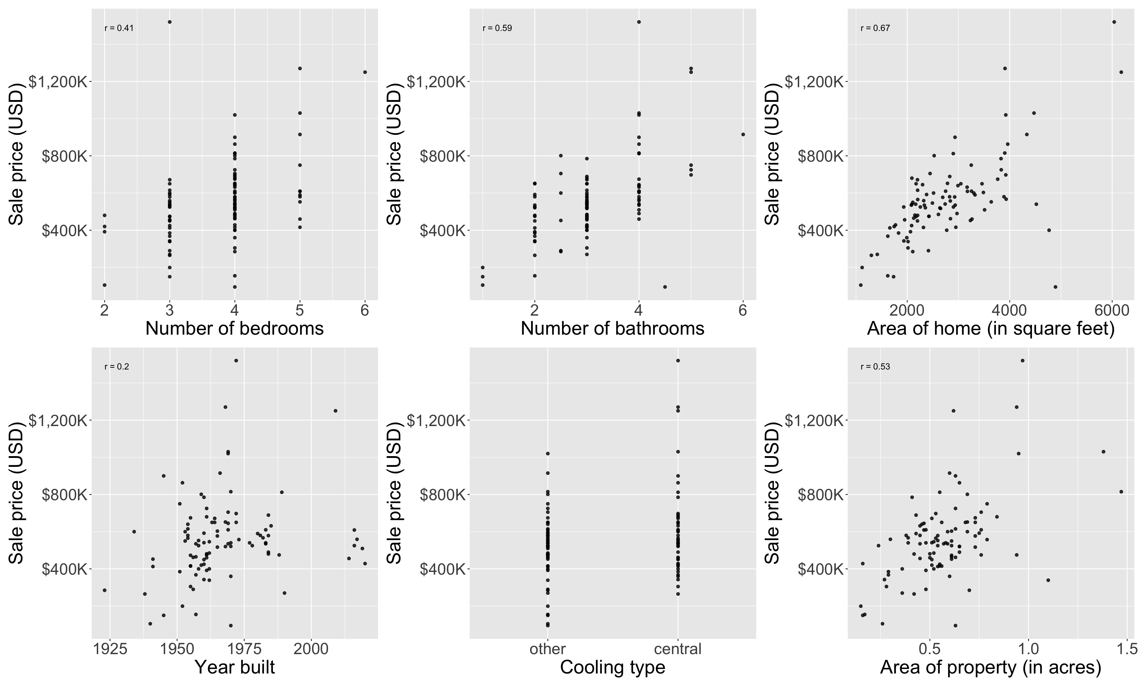
Seems all variables are positively associated with price

Example: housing prices

Let’s now try to predict price from area: single linear regression

lm(price ~ area, data = duke_forest) |> broom::tidy() |> kable(digits=2)

term	estimate	std.error	statistic	p.value
(Intercept)	116652.33	53302.46	2.19	0.03
area	159.48	18.17	8.78	0.00

This gives the predictive model \[ \widehat{\mathsf{price}} = 116,652 + 159\times \mathsf{area}\]
Each additional increase in area by one square foot is expected to increase a home’s price by $159

Does appear to be a linear relationship, but residuals for expensive homes are quite large. Not clear that a linear model is the best model for large/expensive homes, need more advanced methods.

Modeling price with multiple variables

Now model price w/ multiple variables

m_full <- lm(price ~ area + bed + bath + year_built + cooling + lot, data = duke_forest)
m_full |> broom::tidy() |> kable(digits=0)

term	estimate	std.error	statistic	p.value
(Intercept)	-2910715	1787934	-2	0
area	102	23	4	0
bed	-13692	25928	-1	1
bath	41076	24662	2	0
year_built	1459	914	2	0
coolingcentral	84065	30338	3	0
lot	356141	75940	5	0

This forms the predictive model

\[\begin{align} \widehat{\texttt{price}} &= -2,910,715 \\ &\quad+ 102 \times \texttt{area} \\ &\quad- 13,692 \times \texttt{bed} \\ &\quad+ 41,076 \times \texttt{bath} \\ &\quad+ 1,459 \times \texttt{year_built}\\ &\quad+ 84,065 \times \texttt{cooling}_{\texttt{central}} \\ &\quad+ 356,141 \times \texttt{lot} \end{align}\]

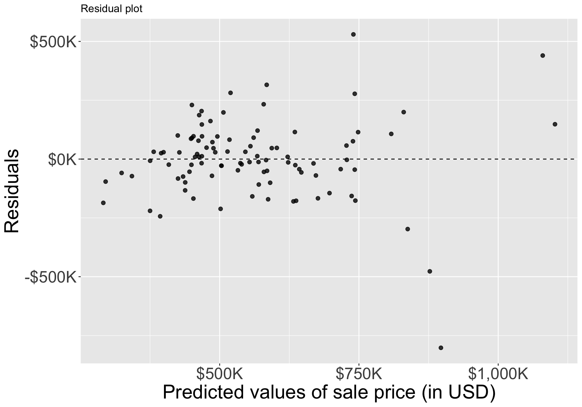
Modeling price with multiple variables

Residuals appear to be randomly scattered around zero, but again pretty large residuals for expensive homes
One apparent outlier at $-\$750K$ predicted value.

Backward elimination

Let’s see if excluding certain variables helps to improve the model’s $R^2_{adj}$
Helpful function in R: update()
Takes lm() output and allows you to specify what changes you’d like to make
. ~ . - variable <–> use same formula as before, but now remove variable from the formula

update(m_full, . ~ . - area, 
       data = duke_forest) |> 
  broom::tidy() |>
  kable(digits=0)

term	estimate	std.error	statistic	p.value
(Intercept)	-3056731	1960957	-2	0
bed	15103	27528	1	1
bath	91076	24034	4	0
year_built	1521	1002	2	0
coolingcentral	67210	33015	2	0
lot	447962	80120	6	0

model summary omits area

Backward elimination

m_full |> broom::glance() |> pull(adj.r.squared)

[1] 0.5896359

Baseline $R^2_{adj}$ from the full model is 0.5896.

Will dropping a predictor improve $R^2_{adj}$?

# Compute adjusted R^2 for model `m_full` 
# after removing predictor `area`
update(m_full, . ~ . - area, 
       data = duke_forest) |> 
  glance() |> 
  pull(adj.r.squared)

[1] 0.5062002

Excluding area: 0.5062
Excluding bed: 0.5929
Excluding bath: 0.5816
Excluding year_built: 0.5826
Excluding cooling: 0.5595
Excluding lot: 0.4894

Backward elimination

Excluding bed improves adjusted $R^2$, so we eliminate this
- Excluding bed and area: 0.506
- Excluding bed and bath: 0.586
- Excluding bed and year_built: 0.586
- Excluding bed and cooling: 0.563
- Excluding bed and lot: 0.493
None of these improve on the (new) baseline adjusted $R^2$ of $0.593$, so we don’t change the model any more

Backward elimination

Removing bed, we have the following model:

m_full <- lm(price ~ area + bed + bath + year_built + cooling + lot, data = duke_forest)
update(m_full, . ~ . - bed, data = duke_forest) |> broom::tidy()

# A tibble: 6 × 5
  term             estimate std.error statistic    p.value
  <chr>               <dbl>     <dbl>     <dbl>      <dbl>
1 (Intercept)    -2952641.  1779079.      -1.66 0.100     
2 area                 99.1      22.3      4.44 0.0000249 
3 bath              36228.    22799.       1.59 0.116     
4 year_built         1466.      910.       1.61 0.111     
5 coolingcentral    83856.    30215.       2.78 0.00669   
6 lot              357119.    75617.       4.72 0.00000841

\[ \begin{aligned} \widehat{\texttt{price}} &= -2,952,641 + 99 \times \texttt{area}\\ &+ 36,228 \times \texttt{bath} + 1,466 \times \texttt{year_built}\\ &+ 83,856 \times \texttt{cooling}_{\texttt{central}} + 357,119 \times \texttt{lot} \end{aligned} \]

Automate this process

Backward elimination and forward selection are widely taught and have been around for a long time

We stepped through this process to learn and understand the procedure
Calculations and selections have been implemented in e.g., R package olsrr

# install.packages("olsrr")
library(olsrr)
surgical |> head(3)

  bcs pindex enzyme_test liver_test age gender alc_mod alc_heavy   y
1 6.7     62          81       2.59  50      0       1         0 695
2 5.1     59          66       1.70  39      0       0         0 403
3 7.4     57          83       2.16  55      0       0         0 710

model <- lm(y ~ ., data = surgical)

See olsrr vignette for more information about package

Automate this process: Backward elimination

# stepwise backward regression
ols_step_backward_p(model)


                             Stepwise Summary                              
-------------------------------------------------------------------------
Step    Variable        AIC        SBC       SBIC        R2       Adj. R2 
-------------------------------------------------------------------------
 0      Full Model    736.390    756.280    586.665    0.78184    0.74305 
 1      alc_mod       734.407    752.308    584.276    0.78177    0.74856 
 2      gender        732.494    748.406    581.938    0.78142    0.75351 
 3      age           730.620    744.543    579.638    0.78091    0.75808 
-------------------------------------------------------------------------

Final Model Output 
------------------

                           Model Summary                            
-------------------------------------------------------------------
R                         0.884       RMSE                 184.276 
R-Squared                 0.781       MSE                33957.712 
Adj. R-Squared            0.758       Coef. Var             27.839 
Pred R-Squared            0.700       AIC                  730.620 
MAE                     137.656       SBC                  744.543 
-------------------------------------------------------------------
 RMSE: Root Mean Square Error 
 MSE: Mean Square Error 
 MAE: Mean Absolute Error 
 AIC: Akaike Information Criteria 
 SBC: Schwarz Bayesian Criteria 

                                 ANOVA                                  
-----------------------------------------------------------------------
                   Sum of                                              
                  Squares        DF    Mean Square      F         Sig. 
-----------------------------------------------------------------------
Regression    6535804.090         5    1307160.818    34.217    0.0000 
Residual      1833716.447        48      38202.426                     
Total         8369520.537        53                                    
-----------------------------------------------------------------------

                                      Parameter Estimates                                        
------------------------------------------------------------------------------------------------
      model         Beta    Std. Error    Std. Beta      t        Sig         lower       upper 
------------------------------------------------------------------------------------------------
(Intercept)    -1178.330       208.682                 -5.647    0.000    -1597.914    -758.746 
        bcs       59.864        23.060        0.241     2.596    0.012       13.498     106.230 
     pindex        8.924         1.808        0.380     4.935    0.000        5.288      12.559 
enzyme_test        9.748         1.656        0.521     5.887    0.000        6.419      13.077 
 liver_test       58.064        40.144        0.156     1.446    0.155      -22.652     138.779 
  alc_heavy      317.848        71.634        0.314     4.437    0.000      173.818     461.878 
------------------------------------------------------------------------------------------------

Automate this process: Forward selection

# stepwise forward regression
ols_step_forward_p(model)


                              Stepwise Summary                              
--------------------------------------------------------------------------
Step    Variable         AIC        SBC       SBIC        R2       Adj. R2 
--------------------------------------------------------------------------
 0      Base Model     802.606    806.584    646.794    0.00000    0.00000 
 1      liver_test     771.875    777.842    616.009    0.45454    0.44405 
 2      alc_heavy      761.439    769.395    605.506    0.56674    0.54975 
 3      enzyme_test    750.509    760.454    595.297    0.65900    0.63854 
 4      pindex         735.715    747.649    582.943    0.75015    0.72975 
 5      bcs            730.620    744.543    579.638    0.78091    0.75808 
--------------------------------------------------------------------------

Final Model Output 
------------------

                           Model Summary                            
-------------------------------------------------------------------
R                         0.884       RMSE                 184.276 
R-Squared                 0.781       MSE                33957.712 
Adj. R-Squared            0.758       Coef. Var             27.839 
Pred R-Squared            0.700       AIC                  730.620 
MAE                     137.656       SBC                  744.543 
-------------------------------------------------------------------
 RMSE: Root Mean Square Error 
 MSE: Mean Square Error 
 MAE: Mean Absolute Error 
 AIC: Akaike Information Criteria 
 SBC: Schwarz Bayesian Criteria 

                                 ANOVA                                  
-----------------------------------------------------------------------
                   Sum of                                              
                  Squares        DF    Mean Square      F         Sig. 
-----------------------------------------------------------------------
Regression    6535804.090         5    1307160.818    34.217    0.0000 
Residual      1833716.447        48      38202.426                     
Total         8369520.537        53                                    
-----------------------------------------------------------------------

                                      Parameter Estimates                                        
------------------------------------------------------------------------------------------------
      model         Beta    Std. Error    Std. Beta      t        Sig         lower       upper 
------------------------------------------------------------------------------------------------
(Intercept)    -1178.330       208.682                 -5.647    0.000    -1597.914    -758.746 
 liver_test       58.064        40.144        0.156     1.446    0.155      -22.652     138.779 
  alc_heavy      317.848        71.634        0.314     4.437    0.000      173.818     461.878 
enzyme_test        9.748         1.656        0.521     5.887    0.000        6.419      13.077 
     pindex        8.924         1.808        0.380     4.935    0.000        5.288      12.559 
        bcs       59.864        23.060        0.241     2.596    0.012       13.498     106.230 
------------------------------------------------------------------------------------------------

Automate this process: make it prettier

ols_step_forward_p(model)$metrics |> 
    select(step, variable, adj_r2) |> 
    kable(digits=3)

step	variable	adj_r2
1	liver_test	0.444
2	alc_heavy	0.550
3	enzyme_test	0.639
4	pindex	0.730
5	bcs	0.758

Make prettier by changing adj_r2 to “Adjusted $R^2$”, etc.
Function kable() comes from package kableExtra.
See package kableExtra for more functionality.

Final comments on model selection

There are many commonly used model selection strategies.

E.g., stepwise selection can also be carried out with decision criteria other than adjusted $R^2$ such as p-values, or AIC (Akaike information criterion), or BIC (Bayesian information criterion), which you might learn about in more advanced courses.
Alternatively, one could include / exclude predictors from a model based on expert opinion or due to research focus.
- Many statisticians discourage the use of stepwise regression alone for model selection and advocate, instead, for a more thoughtful approach that carefully considers the research focus and features of the data.