library(ggplot2)library(tidyverse)library(unvotes)library(knitr)library(scales)library(ggpubr) # for statcor()library(broom) # for tidy()library(openintro)library(patchwork)
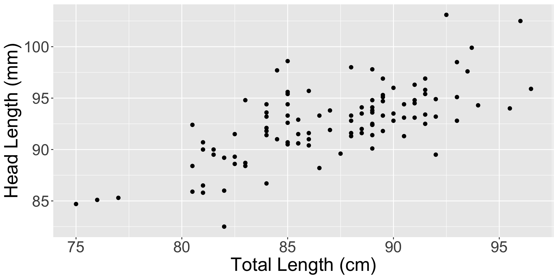
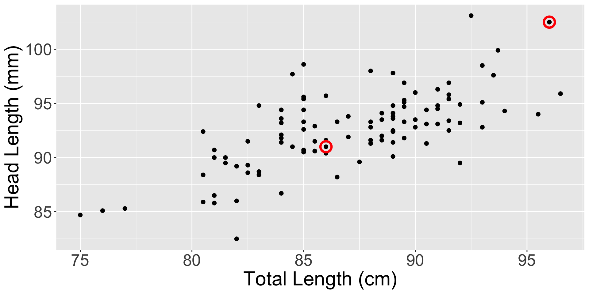
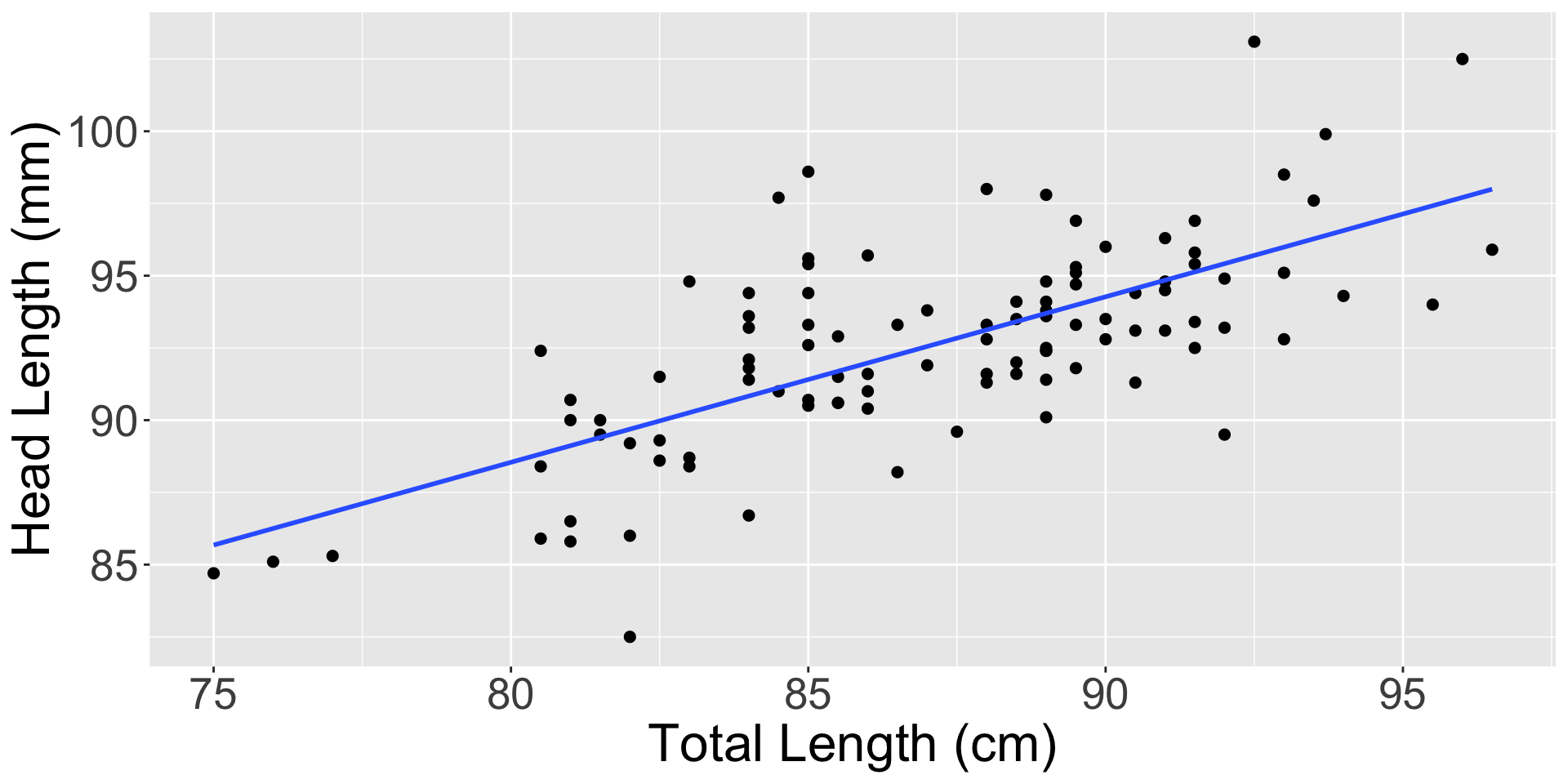
Figure 1: A scatterplot showing head length against total length for 104 brushtail possums. A point representing a possum with head length 86.7 mm and total length 84 cm is highlighted.
Recall from algebra…
A quick refresher on plotting lines:
“Slope-intercept form” with slope \(m\) and intercept \(b\): \[y = m x + b\]
“Point-slope form”: a line going through \((x_0, y_0)\) with slope \(m\) is \[y - y_0 = m (x - x_0)\]
If you have two points, you can always connect a line through them and find the slope by substituting into first equation above.
Linear model
A linear model is a general framework that describes a linear relationship between a dependent variable and one or more independent variables.
For this slide deck, assume just one predictor variable
Linear model
Why model the relationship as linear?
Easy math, compute, interpret
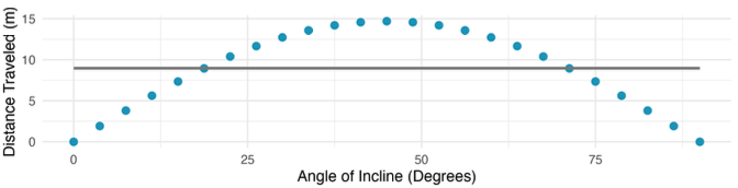
Also cases where fitting a line to the data, even if there is a clear relationship between the variables, is not helpful. (Discuss nonlinear trends later)
The best fitting line for these data is flat; not useful for describing this clear non-linear relationship. These data are from a physics experiment.
Linear regression
How do we fit a “good” line to the data?
Linear regression: the statistical method for fitting a line to data for variables in a linear model.
Because a line is defined by a slope and intercept, we thus want to learn/estimate the slope and intercept of the linear relationship
However, a perfect explanatory relationship (linear or not) is unrealistic in almost any natural process.
Causes: observation noise, missing mechanisms, etc.
In such cases, data will not fall perfectly onto a line (See Figure 1)
We thus also want to capture the errors (deviations from linear relationship)
Basic single-variable linear model
The basic structure of a linear model: \[ y = b_0 + b_1 x + \epsilon \]
\(b_0\) is intercept, \(b_1\) is slope, \(\epsilon\) is an error term
We call \(x\) the predictor, \(y\) the response or outcome.
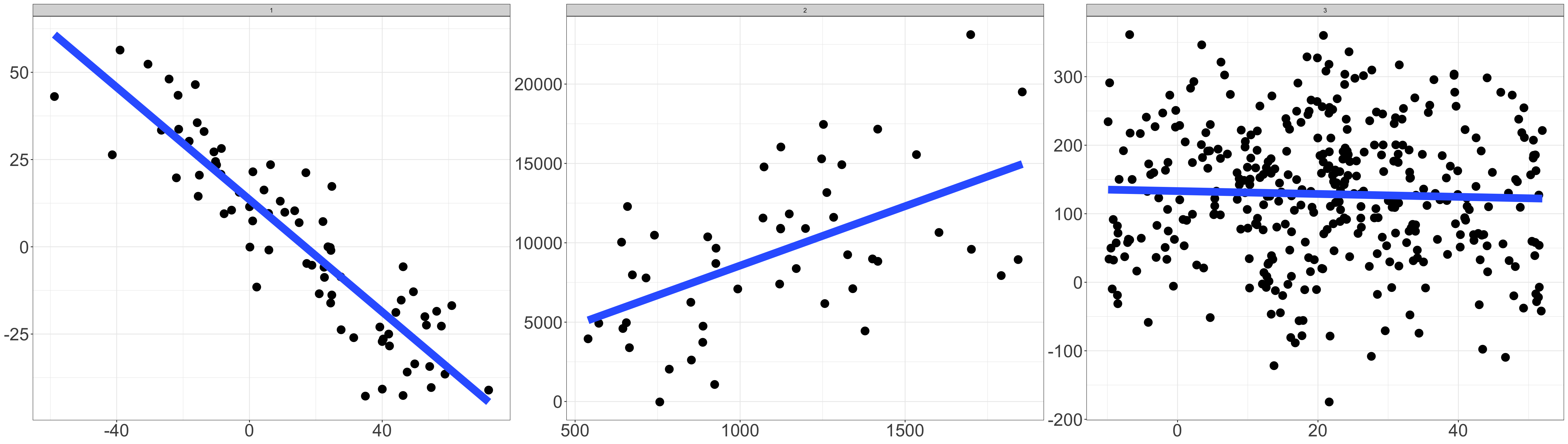
The error term can be small or large — its size relative to the slope determines how useful the linear model is.
Figure 2: Three datasets where a linear model may be useful even if the data do not all fall exactly on the line.
Predicting possum head lengths: fitting a line
We can try and fit a line which roughly fits the data well by randomly picking two points and then drawing the line between them. (not ideal)
ggplot(possum, aes(x = total_l, y = head_l)) +geom_point(alpha =1, size =2) +labs(x ="Total Length (cm)", y ="Head Length (mm)") +geom_point(data =sample_n(possum, 2), aes(x = total_l, y = head_l), color ="red", size =5, shape ="circle open", stroke =2)
Predicting possum head lengths: fitting a line
A more reasonable line:
ggplot(possum, aes(x = total_l, y = head_l)) +geom_point(alpha =1, size =2) +labs(x ="Total Length (cm)", y ="Head Length (mm)") +geom_smooth(method ="lm", se =FALSE)
Predicting possum head lengths: fitting a line
We saw two lines. Which line fits the data better?
Could eyeball, but how to quantify if a fit is “good”? Introduce residuals.
Residuals are the leftover variation in the data after accounting for the model fit: \[\text{Data= Fit + Residual}\] One goal in picking the right linear model is for residuals to be as small as possible.
Residuals
Suppose we fit a line to the data \((x_i, y_i)_{i=1}^n\).
We can make a prediction \(\hat{y}(x) = \hat y\) at any location \(x\). The prediction will simply be the line’s \(y\) value at \(x\).
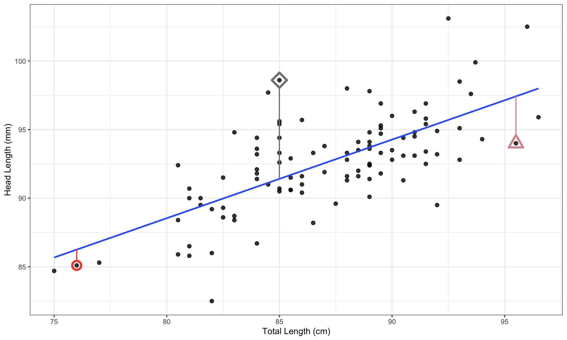
The residual for the \(i\)-th observation \((x_i, y_i)\) is the difference between observed outcome \(y_i\) and predicted outcome \(\hat{y}(x_i) = \hat y_i\): \[ e_i := y_i - \hat y_i .\]
The residual is the vertical length of the line from the line to the point.
Dot above line \(\Rightarrow\) positive residual
Dot below line \(\Rightarrow\) negative residual
Residuals
Example calculation: if the line is given by the equation \[ \hat y = 41 + 0.59 x \] then the residual for the observation \((x_0,y_0) = (76.0, 85.1)\) is \[ \hat y_0 = 41 + 0.59 \times 85.1 = 85.84 \]\[ e_0 = y_0 - \hat y_0 = 85.1 - 85.84 = -0.74 \]
Residuals
… are helpful when trying to understand how well a linear model fits the data
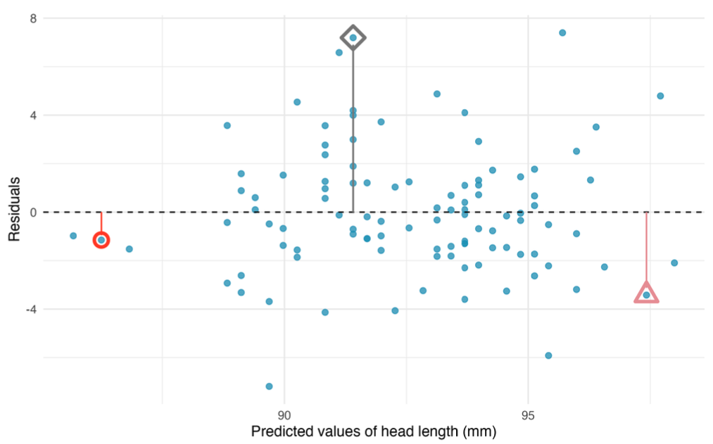
Visualize this by plotting predicted values on \(x\)-axis, and residuals on \(y\)-axis
Residual plot for the model predicting head length from total length for brushtail possums.
Least squares regression
Least squares regression
Return to earlier question: which line fits the data better? More generally, what is the “best” line (if it exists)?
Mathematically, we want a line that has small residuals.
Option 1: choose the line that minimizes the sum of the residual magnitudes: \[|e_1| + |e_2| + \cdots + |e_n|.\]
Option 2: choose the line that minimizes the sum of the squared residuals: \[e_1^2 + e_2^2 + \cdots + e_n^2.\]
Use software to compute the slope and intercept of these lines.
Least squares regression
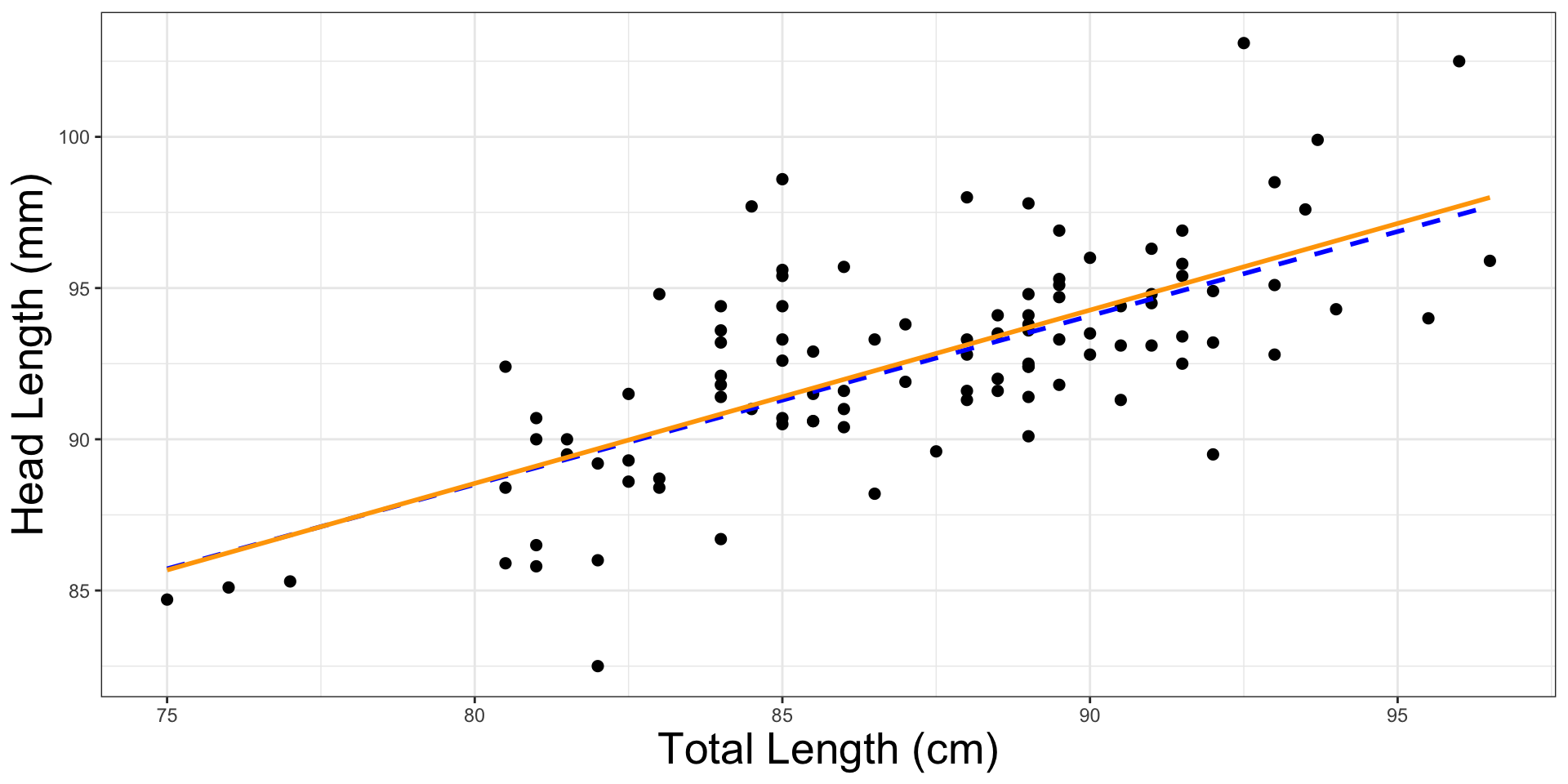
Let’s see these what these two lines look like:
model_rlm <- MASS::rlm(head_l ~ total_l, data = possum) # for LAD Lineggplot(possum, aes(x = total_l, y = head_l)) +geom_point(size =2) +geom_smooth(aes(y =predict(model_rlm)), color="blue", linetype="dashed") +# LAD Linegeom_smooth(method ="lm", se =FALSE, color="orange", linetype="solid") +# OLS Linelabs(x ="Total Length (cm)", y ="Head Length (mm)") +theme_bw() +theme(axis.title=element_text(size=20))
Least squares regression
Line that minimizes this least squares criterion is called the least squares line. Reasons to use this line over option 1:
It is the most commonly used method.
Computing the least squares line is widely supported in statistical software.
In many applications, a residual twice as large as another residual is more than twice as bad.
For example, being off by 4 is usually more than twice as bad as being off by 2. Squaring the residuals accounts for this discrepancy.
The analyses which link the model to inference about a population are most straightforward when the line is fit through least squares.
The rest of this course will use this option.
Interpreting the least squares line
For possum, we could write the equation of the least squares regression line as \[\widehat{\texttt{head_length}} = \beta_0 + \beta_1 \times \texttt{body_length}\]
\(\beta_0\) and \(\beta_1\) are the population parameters of the linear relationship.
Let’s estimate these population parameters using the observed data.
lm(head_l ~ total_l, data = possum) |> broom::tidy() |>kable()
term
estimate
std.error
statistic
p.value
(Intercept)
42.7097931
5.1728138
8.256588
0
total_l
0.5729013
0.0593253
9.656946
0
estimated intercept is \(\hat\beta_0 \approx 42.7\); estimated slope is \(\hat\beta_1 \approx 0.573\).
The slope describes the estimated difference in the predicted average outcome of \(y\) if the predictor variable \(x\) happened to be one unit larger.
The intercept describes the average outcome of \(y\) if \(x = 0\) and the linear model is valid all the way to \(x = 0\) (values of \(x = 0\) are not observed or relevant in many applications).
In our example: For each additional cm of body length, we would expect a possum’s head to be \(0.573\)mm larger.
Caution: despite this real association, we cannot interpret a causal connection between the variables because these data are observational.
In our example: A possum with no body length is expected to have a head length of \(42.7\)mm. (Here the intercept is not meaningful because there are no observations where \(x\) is near zero. Also, a possum cannot have zero body length.)
Extrapolation is treacherous
Generally speaking, we will not know how data outside of our limited window will behave.
In our data, the range of body lengths is [75, 96.5]. This is far away from \(\texttt{total_l} = 0\), which is (one reason) why our interpretation of the intercept did not make sense.
Applying a model estimate to values outside of the realm of the original data is called extrapolation.
If we extrapolate, we make an unreliable bet that the estimated relationship will be valid in unobserved places.
Describing the strength of a linear fit: correlation
Can we quantify the strength of a linear relationship with a single statistic?
Before we introduce correlation, let’s recall some basic summary statistics:
Suppose we want to summarize a set of values \(a_1,a_2,\ldots,a_n\).
We can quantify a “representative value” using sample meanmean(): \[\bar{a} = \frac{1}{n} \sum_{i=1}^n a_i.\]
or sample standard deviationsd(): \[s_a = \sqrt{s_a^2}\]
Describing the strength of a linear fit: correlation
Can we quantify the strength of a linear relationship with a single statistic?
The correlation describes the strength and direction of the linear relationship between two variables. For \(n\) data points, the correlation is defined as \[r = \frac{1}{n-1} \sum_{i=1}^n \frac{x_i - \bar{x}}{s_x} \frac{y_i - \bar{y}}{s_y}\] where \(\bar{x}\), \(\bar{y}\), \(s_x\), and \(s_y\) are the sample means and standard deviations for each variable.
It is always a value between -1 and 1.
It is unitless; it will not be affected by a linear change in the units (e.g., going from inches to centimeters).
Describing the strength of a linear fit: correlation
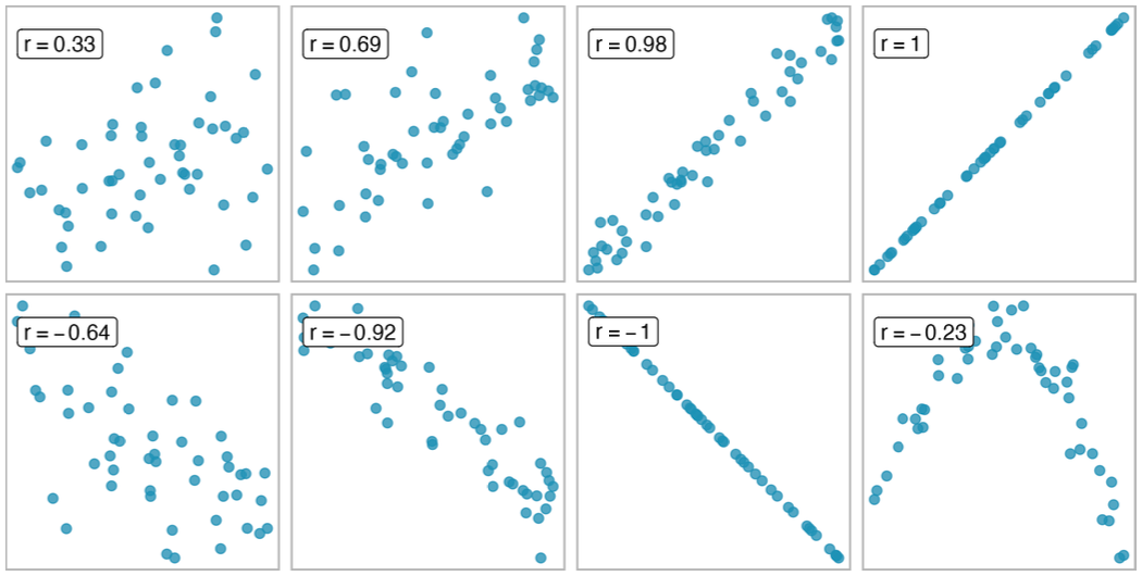
Sample scatterplots and their correlations. The first row shows variables with a positive relationship, represented by the trend up and to the right. The second row shows variables with a negative trend, where a large value in one variable is associated with a lower value in the other.
Describing the strength of a linear fit: correlation
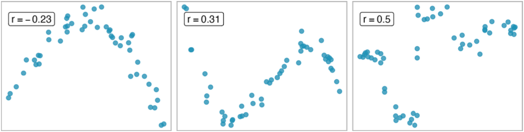
Sample scatterplots and their correlations. In each case, there is a strong relationship between the variables. However, because the relationship is not linear, the correlation is relatively weak.
Describing the strength of a linear fit: \(R^2\)
Common to use \(R^2\), called R-squared or coefficient of determination:
describes how closely the data cluster around the linear fit
describes the amount of variation in the outcome variable that is explained by the least squares line.
var(possum$head_l) # Variance of the response variable, i.e., total sum of squares (SST)
[1] 12.76883
var(possum$head_l -predict(lm(head_l ~ total_l, possum))) # Variance of the residuals, i.e. sum of squared errors (SSE)
[1] 6.670301
1-var(possum$head_l -predict(lm(head_l ~ total_l, possum))) /var(possum$head_l) # R^2: proportion of response variable's variation explained by least squares line. R^2 = (1 - SSE / SST)
[1] 0.4776105
cor(possum$head_l, possum$total_l) ^2# squared value of the correlation; same value as R^2
[1] 0.4776105
Describing the strength of a linear fit: \(R^2\)
Total sum of squares: variability in the \(y\) values about their mean, \(\bar{y}\)\[SST = (y_1 - \bar{y})^2 + (y_2 - \bar{y})^2 + \cdots + (y_n - \bar{y})^2\]
Sum of squared errors (or sum of squared residuals): variability in residuals \[SSE = (y_1 - \hat{y}_1)^2 + (y_2 - \hat{y}_2)^2 + \cdots + (y_n - \hat{y}_n)^2\]
The coefficient of determination, \(R^2\), can then be calculated as \[R^2 = 1 - \frac{SSE}{SST}\]
Turns out to be equivalent to the squared value of the correlation
Interpretation for possum: \(R^2 = 0.48\) or \(48\%\) of the variation in head_l is explained by the linear model.
Categorical predictors with two levels
So far we have used continuous (numeric) predictor variables.
Categorical variables are also useful in predicting outcomes.
Categorical predictors with two levels
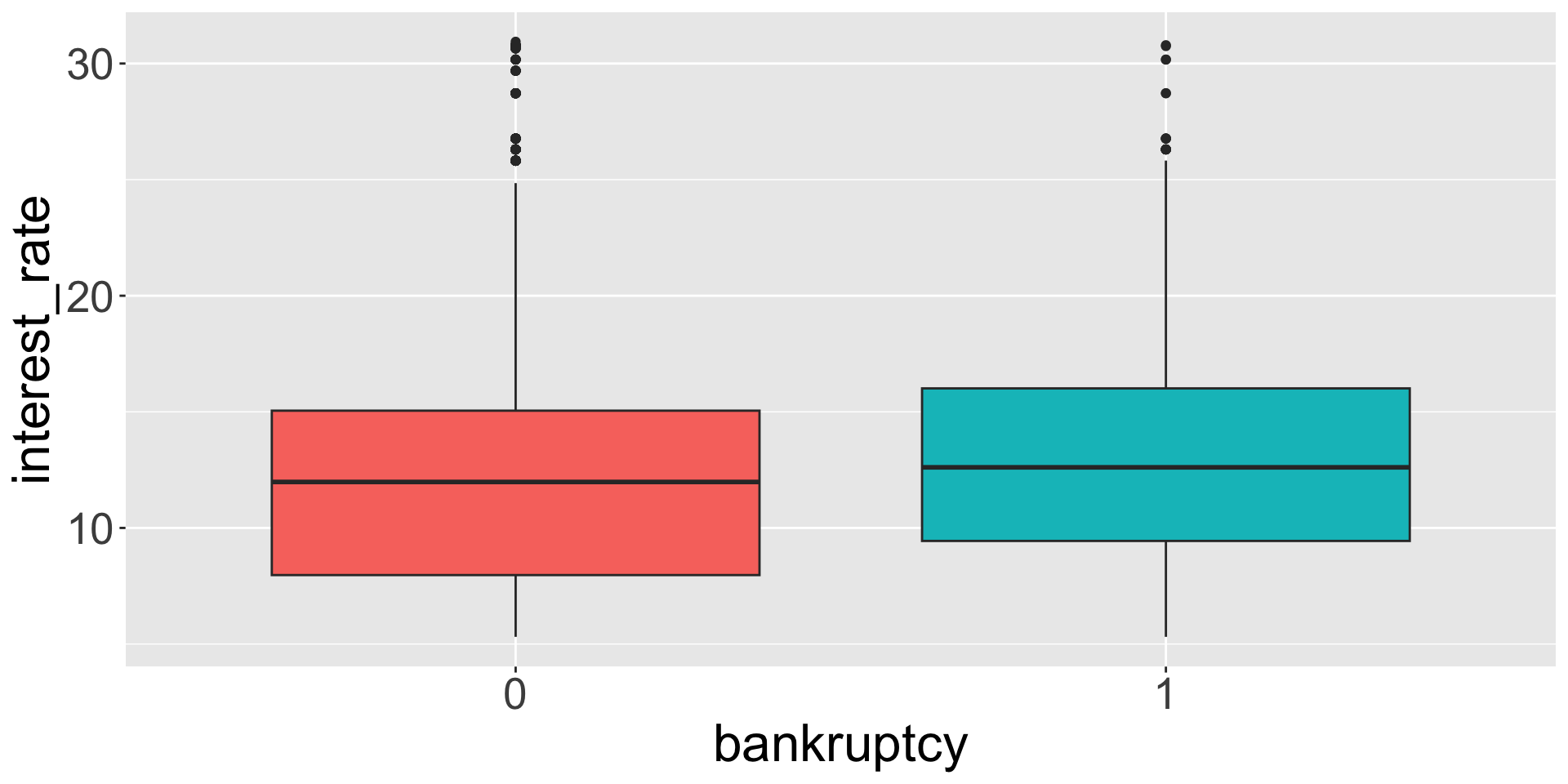
Example: Predict the interest rate for someone based on whether that person has filed for bankruptcy. (Data from openintro::loans_full_schema.)
Seems plausible that bankruptcy is associated with a higher interest rate
Categorical predictors with two levels
Let’s inspect the least-squares linear model resulting from this
lm(interest_rate ~ bankruptcy, data = loans) |> broom::tidy() |>kable()
term
estimate
std.error
statistic
p.value
(Intercept)
12.3380046
0.0532983
231.489782
0.0e+00
bankruptcy1
0.7367856
0.1529062
4.818548
1.5e-06
Average interest rate is \(12.34 \%\) for those w/o bankruptcy
Model predicts \(0.74\%\) higher interest rate for those w/ bankruptcy
Average interest rate is \(12.34 \% + 0.74\% = 13.08\%\) for those w/ bankruptcy
Fundamentally, the intercept and slope interpretations do not change when modeling categorical variables with two levels.
Outliers in linear regression
Outliers in linear regression
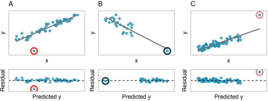
An outlier is an observation \((x,y)\) that falls far from the bivariate model.
Outliers can have a strong influence on the least squares line: if we remove an outlier, how much does the line of best fit change?
Good practice for dealing with outlying observations is to produce two analyses: one with and one without the outlying observations.
Provides insight into role of outlying observations and subsequent appropriate model.
Outliers in linear regression
Points that fall horizontally away from the center of the cloud tend to pull harder on the line, so we call them points with high leverage or leverage points.
These points can strongly influence the slope of the least squares line.
If such a point does seem to have a strong influence, call it an influential point.
It is tempting to remove outliers. Don’t do this without a very good reason. Models that ignore exceptional (and interesting) cases often perform poorly.