s3: exploring data using tidyverse

STA141A: Fundamentals of Statistical Data Science

Akira Horiguchi

Quick note

Wickham and Grolemund (2017)

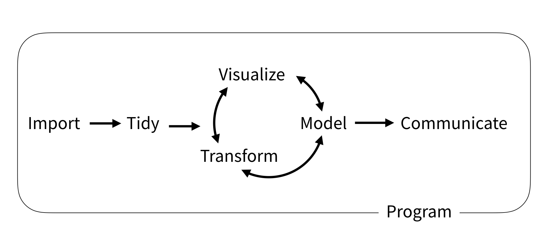
This slide deck (3-4 lectures) is meant to get you started working with data: Import, Tidy, Transform, Visualize. (Modeling will be middle half of this course.)

By no means is it exhaustive.
Too much? Too little? Strongly depends on previous experience.
PRACTICE with basic tools to get comfortable before learning new ones.

`tidyverse`

`tidyverse` approach to data manipulation

Why use tidyverse over base R or data.table or other packages?

The tidyverse is an opinionated collection of R packages designed for data science. All packages share an underlying design philosophy, grammar, and data structures. — https://www.tidyverse.org/

Consistent syntax.
Many people work full-time (and get paid!) to make new packages, add new functionality, etc.
- In contrast, many other packages are created/maintained/updated by researchers who work on this part-time.
Downside: slow for large data sets. (Use data.table instead.)

This slide deck will primarily use tidyverse solutions, but it’s always good to know base R solutions.

Reminder about packages

Packages are things we load using library().
If you haven’t installed a package PACKAGENAME before, you’ll get an error.
To install a package: install.packages("PACKAGENAME").
To load a package: library(PACKAGENAME).
For example:

install.packages("tidyverse")  # Do just once
library(tidyverse)  # Do at the start of every session

Load example dataset

library(nycflights13) # loads the `flights` tibble into environment
flights

# A tibble: 336,776 × 19
    year month   day dep_time sched_dep_time dep_delay arr_time sched_arr_time
   <int> <int> <int>    <int>          <int>     <dbl>    <int>          <int>
 1  2013     1     1      517            515         2      830            819
 2  2013     1     1      533            529         4      850            830
 3  2013     1     1      542            540         2      923            850
 4  2013     1     1      544            545        -1     1004           1022
 5  2013     1     1      554            600        -6      812            837
 6  2013     1     1      554            558        -4      740            728
 7  2013     1     1      555            600        -5      913            854
 8  2013     1     1      557            600        -3      709            723
 9  2013     1     1      557            600        -3      838            846
10  2013     1     1      558            600        -2      753            745
# ℹ 336,766 more rows
# ℹ 11 more variables: arr_delay <dbl>, carrier <chr>, flight <int>,
#   tailnum <chr>, origin <chr>, dest <chr>, air_time <dbl>, distance <dbl>,
#   hour <dbl>, minute <dbl>, time_hour <dttm>

Piping

The pipe operator %>% (requires the magrittr package) allow you to write operations sequentially.

mean(flights$distance)

[1] 1039.913

Can instead pipe an output into the (first) argument of another function.

flights$distance %>%
  mean()

[1] 1039.913

Can also use |>, which is included in R 4.1.0 (no need to install another package)

Piping

Why pipe? Can be easier to read and understand.

mean(sqrt(log(flights$distance)))  # somewhat difficult to read

[1] 2.580285

flights$distance |>  # easier to read
  log() |>
  sqrt() |>
  mean()

[1] 2.580285

We will see more complex examples of this shortly.

Importing data

Introduction

We have seen data sets that are either built into base R or come from external packages

We will eventually want to import data from external files

Types of data files

CSV: comma separated values (this course will use this type the most)
TSV: tab separated values
FWF: fixed width file

To load files, the readr package has the following functions:

read_csv(), read_tsv(), read_delim()
read_fwf(), read_table()

`read_csv()`: can you spot the differences?

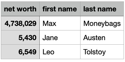
networth.csv

read.csv("networth.csv")  # from utils package; preinstalled with R

  net.worth first.name last.name
1 4,738,029        Max Moneybags
2     5,430       Jane    Austen
3     6,549        Leo   Tolstoy

read_csv("networth.csv")  # from readr package

# A tibble: 3 × 3
  `net worth` `first name` `last name`
        <dbl> <chr>        <chr>      
1     4738029 Max          Moneybags  
2        5430 Jane         Austen     
3        6549 Leo          Tolstoy

`read_csv()`: can you spot the differences?

Column names can have spaces. How to access?

nw_df <- read_csv("networth.csv")
nw_df

# A tibble: 3 × 3
  `net worth` `first name` `last name`
        <dbl> <chr>        <chr>      
1     4738029 Max          Moneybags  
2        5430 Jane         Austen     
3        6549 Leo          Tolstoy

nw_df$`net worth` * 10

[1] 47380290    54300    65490

You’ll likely want to use external files for your final project

For lecture, mostly stick with datasets from base R or packages

Subsetting a data frame

Subset based on data values (rather than row/column indices)

Column: select()
Row: filter()

The `select()` function

Returns a tibble with the columns specified, in order specified.

flights |>
  select(origin, dest, air_time, distance) |>  # Do not need quotation marks.
  colnames()

[1] "origin"   "dest"     "air_time" "distance"

flights |>
  select(distance, dest, origin, air_time) |>  # Do not need quotation marks.
  colnames()

[1] "distance" "dest"     "origin"   "air_time"

colnames(select(flights, distance, dest, origin, air_time))  # hard to read

[1] "distance" "dest"     "origin"   "air_time"

Helper functions for `select()`

starts_with("abc"): matches names that begin with “abc”.
ends_with("xyz"): matches names that end with “xyz”.
contains("ijk"): matches names that contain “ijk”.

flights |> colnames()

 [1] "year"           "month"          "day"            "dep_time"      
 [5] "sched_dep_time" "dep_delay"      "arr_time"       "sched_arr_time"
 [9] "arr_delay"      "carrier"        "flight"         "tailnum"       
[13] "origin"         "dest"           "air_time"       "distance"      
[17] "hour"           "minute"         "time_hour"

flights |> select(origin, dest, contains("sched"))

# A tibble: 336,776 × 4
   origin dest  sched_dep_time sched_arr_time
   <chr>  <chr>          <int>          <int>
 1 EWR    IAH              515            819
 2 LGA    IAH              529            830
...

The `filter()` function

# data = data to filter
# expr<#> = expression used to filter data, typically using ==, >, etc
filter(<data>, <expr1>)
filter(<data>, <expr1>, <expr2>, <expr3>)

Example: flights on February 15

filter(flights, month == 2, day == 15)

# A tibble: 954 × 19
    year month   day dep_time sched_dep_time dep_delay arr_time sched_arr_time
   <int> <int> <int>    <int>          <int>     <dbl>    <int>          <int>
 1  2013     2    15        3           2358         5      503            438
 2  2013     2    15        6           2115       171       48           2214
 3  2013     2    15        6           2250        76      117              5
 4  2013     2    15       22           2230       112      510            312
 5  2013     2    15       36           2352        44      607            437
...

flights |> filter(month == 2, day == 15)  # same as above

The `filter()` function

# data = data to filter
# expr = expression used to filter data, typically using ==, >, etc
filter(<data>, <expr>)

Expressions can be built up using comparison operators and logical operators.

& is “and”
| is “or”
! is “not”
%in% is a membership checker (is an object inside of a vector)
>, < mean greater than, less than
>=, <= mean greater than or equal to, less than or requal to
== means “is equal”
!= means “is not equal”

Examples of `filter()`

flights |>
  select(time_hour, origin, dest, air_time, distance) |>
  filter(distance < 120)

# A tibble: 2,076 × 5
   time_hour           origin dest  air_time distance
   <dttm>              <chr>  <chr>    <dbl>    <dbl>
 1 2013-01-01 09:00:00 LGA    PHL         32       96
 2 2013-01-01 13:00:00 EWR    BDL         25      116
 3 2013-01-01 16:00:00 JFK    PHL         35       94
...

flights |>
  select(time_hour, origin, dest, air_time, distance) |>
  filter(distance < 120, origin == 'EWR')

# A tibble: 493 × 5
   time_hour           origin dest  air_time distance
   <dttm>              <chr>  <chr>    <dbl>    <dbl>
 1 2013-01-01 13:00:00 EWR    BDL         25      116
 2 2013-01-01 22:00:00 EWR    BDL         24      116
...

Spot the error?

flights |>
  select(origin, dest, air_time, distance) |>
  filter(origin == SFO)

Spot the error?

flights |>
  select(origin, dest, air_time, distance) |>
  filter(origin == 'SFO')

Equivalent ways to filter on multiple conditions

flights |>
  select(origin, dest, air_time, distance) |>
  filter(distance < 120, origin == "EWR")

# A tibble: 493 × 4
   origin dest  air_time distance
   <chr>  <chr>    <dbl>    <dbl>
 1 EWR    BDL         25      116
 2 EWR    BDL         24      116
 3 EWR    BDL         24      116
...

flights |>
  select(origin, dest, air_time, distance) |>
  filter(distance < 120 & origin == "EWR")

flights |>
  select(origin, dest, air_time, distance) |>
  filter(distance < 120) |>
  filter(origin == "EWR")

Inspect a data frame

`count()`

To count occurrences of each unique value in a column:

dataframe |>
  count(column1, ...)

e.g., want to count how many flights by origin:

flights |>
  count(origin)

# A tibble: 3 × 2
  origin      n
  <chr>   <int>
1 EWR    120835
2 JFK    111279
3 LGA    104662

Can also count occurrences for multiple columns:

flights |>
  count(origin, dest)

# A tibble: 224 × 3
   origin dest      n
   <chr>  <chr> <int>
 1 EWR    ALB     439
 2 EWR    ANC       8
 3 EWR    ATL    5022
 4 EWR    AUS     968
 5 EWR    AVL     265
 6 EWR    BDL     443
 7 EWR    BNA    2336
 8 EWR    BOS    5327
 9 EWR    BQN     297
10 EWR    BTV     931
# ℹ 214 more rows

`count()`

To count occurrences of each unique value in a column:

dataframe |>
  count(column1, ...)

e.g., want to count how many flights by origin:

flights |>
  count(origin)

# A tibble: 3 × 2
  origin      n
  <chr>   <int>
1 EWR    120835
2 JFK    111279
3 LGA    104662

Can also count occurrences for multiple columns:

flights |>
  count(origin, dest, sort=TRUE)

# A tibble: 224 × 3
   origin dest      n
   <chr>  <chr> <int>
 1 JFK    LAX   11262
 2 LGA    ATL   10263
 3 LGA    ORD    8857
 4 JFK    SFO    8204
 5 LGA    CLT    6168
 6 EWR    ORD    6100
 7 JFK    BOS    5898
 8 LGA    MIA    5781
 9 JFK    MCO    5464
10 EWR    BOS    5327
# ℹ 214 more rows

Summary statistics and missing data

Common summary statistics of interest in data:

Mean (mean())
Min/max (min(), max())
Median (median())
Standard deviation / variance (sd(), var())

R denotes missing data using NA. Typically, if you compute a function of a vector with NAs, it will return NA, unless you put na.rm=TRUE.

x <- c(-1, 0, 1, NA)
mean(x)

[1] NA

mean(x, na.rm=TRUE)

[1] 0

`summarise()`

If you want to compute summary statistics of dataframe, use summarise().

# data = data you want to create a new variable from
# new var name = the name your new variable will be
# calc exp = the calculation you want to perform
summarise(<data>, <new var name> = <calc exp>)

flights |>
  summarise(avg_dist = mean(distance))

# A tibble: 1 × 1
  avg_dist
     <dbl>
1    1040.

Computes summary for the entire dataset

`summarize()`

If you want to compute summary statistics of dataframe, use summarize().

# data = data you want to create a new variable from
# new var name = the name your new variable will be
# calc exp = the calculation you want to perform
summarize(<data>, <new var name> = <calc exp>)

flights |>
  summarize(avg_dist = mean(distance))

# A tibble: 1 × 1
  avg_dist
     <dbl>
1    1040.

Computes summary for the entire dataset

`group_by()` and `summarise()`

To compute summary statistics per category, use group_by() first.

flights |>
  summarize(median_distance = median(distance, na.rm=TRUE),
            max_air_time = max(air_time, na.rm=TRUE))

# A tibble: 1 × 2
  median_distance max_air_time
            <dbl>        <dbl>
1             872          695

flights |>
  group_by(origin) |>
  summarize(median_distance = median(distance, na.rm=TRUE),
            max_air_time = max(air_time, na.rm=TRUE))

# A tibble: 3 × 3
  origin median_distance max_air_time
  <chr>            <dbl>        <dbl>
1 EWR                872          695
2 JFK               1069          691
3 LGA                762          331

`group_by()` and `summarise()`

To compute summary statistics per category, use group_by() first.

flights |>
  summarize(median_distance = median(distance, na.rm=TRUE),
            max_air_time = max(air_time, na.rm=TRUE))

# A tibble: 1 × 2
  median_distance max_air_time
            <dbl>        <dbl>
1             872          695

flights |>
  group_by(origin, dest) |>  # can group by multiple variables
  summarize(median_distance = median(distance, na.rm=TRUE),
            max_air_time = max(air_time, na.rm=TRUE))

# A tibble: 224 × 4
# Groups:   origin [3]
   origin dest  median_distance max_air_time
   <chr>  <chr>           <dbl>        <dbl>
 1 EWR    ALB               143           50
 2 EWR    ANC              3370          434
 3 EWR    ATL               746          176
 4 EWR    AUS              1504          301
 5 EWR    AVL               583          119
 6 EWR    BDL               116           56
 7 EWR    BNA               748          176
 8 EWR    BOS               200          112
 9 EWR    BQN              1585          231
10 EWR    BTV               266           69
# ℹ 214 more rows

`mutate()`

adds new column(s) to the data frame using values from extant columns.

flights |>
  select(air_time, distance, air_time) |>
  mutate(hours = air_time / 60,
         mi_per_hour = distance / hours)

# A tibble: 336,776 × 4
   air_time distance hours mi_per_hour
      <dbl>    <dbl> <dbl>       <dbl>
 1      227     1400 3.78         370.
 2      227     1416 3.78         374.
 3      160     1089 2.67         408.
 4      183     1576 3.05         517.
 5      116      762 1.93         394.
 6      150      719 2.5          288.
...

mi_per_hour uses hours, which was created within the same mutate() call.

`mutate()`

adds new column(s) to the data frame using values from extant columns.

flights |>
  mutate(hours = air_time / 60,
         mi_per_hour = distance / hours, 
         .keep = "used")  # retains only the columns used in creating new columns

# A tibble: 336,776 × 4
   air_time distance hours mi_per_hour
      <dbl>    <dbl> <dbl>       <dbl>
 1      227     1400 3.78         370.
 2      227     1416 3.78         374.
 3      160     1089 2.67         408.
 4      183     1576 3.05         517.
 5      116      762 1.93         394.
 6      150      719 2.5          288.
...

mi_per_hour uses hours, which was created within the same mutate() call.

`mutate()`

adds new column(s) to the data frame using values from extant columns.

flights |>
  mutate(hours = air_time / 60,
         mi_per_hour = distance / hours, 
         .keep = "none")  # retains only grouping variables and the newly created columns

# A tibble: 336,776 × 2
   hours mi_per_hour
   <dbl>       <dbl>
 1 3.78         370.
 2 3.78         374.
 3 2.67         408.
 4 3.05         517.
 5 1.93         394.
 6 2.5          288.
...

mi_per_hour uses hours, which was created within the same mutate() call.

Reshaping a data frame

Tidy data

Multiple equivalent ways of organizing data into a dataframe.

table1
#> # A tibble: 6 × 4
#>   country      year  cases population
#>   <chr>       <dbl>  <dbl>      <dbl>
#> 1 Afghanistan  1999    745   19987071
#> 2 Afghanistan  2000   2666   20595360
#> 3 Brazil       1999  37737  172006362
#> 4 Brazil       2000  80488  174504898
#> 5 China        1999 212258 1272915272
#> 6 China        2000 213766 1280428583

table2
#> # A tibble: 12 × 4
#>   country      year type           count
#>   <chr>       <dbl> <chr>          <dbl>
#> 1 Afghanistan  1999 cases            745
#> 2 Afghanistan  1999 population  19987071
#> 3 Afghanistan  2000 cases           2666
#> 4 Afghanistan  2000 population  20595360
#> 5 Brazil       1999 cases          37737
#> 6 Brazil       1999 population 172006362
#> # ℹ 6 more rows

table1 is tidy - easier to work with using tidyverse.

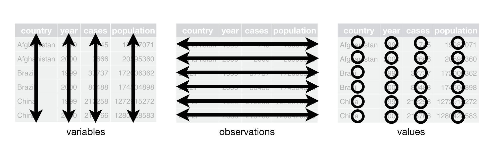
Tidy data

Each variable is a column; each column is a variable.
Each observation is a row; each row is an observation.
Each value is a cell; each cell is a single value.

Tidy data

Why tidy data?

Consistency - uniform format makes collaboration easier
Vectorization - R commands often operate on vectors of data, best for each column to be a vector of data

Tidying data

Unfortunately, most real-world datasets you encounter are NOT tidy.

A large part of “data scientist work” consists in tidying data (“cleaning data”).

billboard

# A tibble: 317 × 79
   artist     track date.entered   wk1   wk2   wk3   wk4   wk5   wk6   wk7   wk8
   <chr>      <chr> <date>       <dbl> <dbl> <dbl> <dbl> <dbl> <dbl> <dbl> <dbl>
 1 2 Pac      Baby… 2000-02-26      87    82    72    77    87    94    99    NA
 2 2Ge+her    The … 2000-09-02      91    87    92    NA    NA    NA    NA    NA
 3 3 Doors D… Kryp… 2000-04-08      81    70    68    67    66    57    54    53
 4 3 Doors D… Loser 2000-10-21      76    76    72    69    67    65    55    59
 5 504 Boyz   Wobb… 2000-04-15      57    34    25    17    17    31    36    49
 6 98^0       Give… 2000-08-19      51    39    34    26    26    19     2     2
 7 A*Teens    Danc… 2000-07-08      97    97    96    95   100    NA    NA    NA
...

Lengthening data with `pivot_longer()`

billboard

# A tibble: 317 × 79
   artist     track date.entered   wk1   wk2   wk3   wk4   wk5   wk6   wk7   wk8
   <chr>      <chr> <date>       <dbl> <dbl> <dbl> <dbl> <dbl> <dbl> <dbl> <dbl>
 1 2 Pac      Baby… 2000-02-26      87    82    72    77    87    94    99    NA
 2 2Ge+her    The … 2000-09-02      91    87    92    NA    NA    NA    NA    NA
 3 3 Doors D… Kryp… 2000-04-08      81    70    68    67    66    57    54    53
...

Each observation is a song.
First three columns (artist, track, date.entered) describe the song.
The next 76 columns (wk1, wk2, …, wk76) say song’s rank in each week.
But week should be a variable.
Each observation should be artist-track-date.entered-week-rank.
To make it tidy, each observation should be a row. Need to make the dataframe longer.

Lengthening data with `pivot_longer()`

billboard |>
  pivot_longer(
    cols = starts_with("wk"),  # `cols`: which columns need to be pivoted
    names_to = "week",  # `names_to`: name of the column that the pivoted column names go
    values_to = "rank"  # `values_to`: name of the column that the pivoted cell values go
  )

# A tibble: 24,092 × 5
   artist track                   date.entered week   rank
   <chr>  <chr>                   <date>       <chr> <dbl>
 1 2 Pac  Baby Don't Cry (Keep... 2000-02-26   wk1      87
 2 2 Pac  Baby Don't Cry (Keep... 2000-02-26   wk2      82
 3 2 Pac  Baby Don't Cry (Keep... 2000-02-26   wk3      72
 4 2 Pac  Baby Don't Cry (Keep... 2000-02-26   wk4      77
...

“week” and “rank” do not appear as column names in billboard, so need quotes

Lengthening data with `pivot_longer()`

billboard |>
  pivot_longer(
    cols = starts_with("wk"),  # `cols`: which columns need to be pivoted
    names_to = "week",  # `names_to`: name of the column that the pivoted column names go
    values_to = "rank"  # `values_to`: name of the column that the pivoted cell values go
  )

# A tibble: 24,092 × 5
   artist track                   date.entered week   rank
   <chr>  <chr>                   <date>       <chr> <dbl>
 1 2 Pac  Baby Don't Cry (Keep... 2000-02-26   wk1      87
 2 2 Pac  Baby Don't Cry (Keep... 2000-02-26   wk2      82
 3 2 Pac  Baby Don't Cry (Keep... 2000-02-26   wk3      72
 4 2 Pac  Baby Don't Cry (Keep... 2000-02-26   wk4      77
...

Data is now tidy, but not ideal for data analysis. Why?

week should ideally be a number, not a character
Can use readr::parse_number() that extracts first number from string to fix.

Lengthening data with `pivot_longer()`

billboard |>
  pivot_longer(
    cols = starts_with("wk"),
    names_to = "week",
    values_to = "rank"
  ) |>
  mutate(week = parse_number(week))

# A tibble: 24,092 × 5
   artist track                   date.entered  week  rank
   <chr>  <chr>                   <date>       <dbl> <dbl>
 1 2 Pac  Baby Don't Cry (Keep... 2000-02-26       1    87
 2 2 Pac  Baby Don't Cry (Keep... 2000-02-26       2    82
 3 2 Pac  Baby Don't Cry (Keep... 2000-02-26       3    72
 4 2 Pac  Baby Don't Cry (Keep... 2000-02-26       4    77
...

Understanding `pivot_longer()`

Consider toy dataset: three people (A, B, C) each with two blood pressure (BP) measurements.

df <- tribble(
  ~id,  ~bp1, ~bp2,
   "A",  100,  120,
   "B",  140,  115,
   "C",  120,  125
)
df

# A tibble: 3 × 3
  id      bp1   bp2
  <chr> <dbl> <dbl>
1 A       100   120
2 B       140   115
3 C       120   125

Want each observation (id, bp) to have its own row:

df |>
  pivot_longer(
    cols = c(bp1, bp2),
    names_to = "measurement",
    values_to = "value"
  )

# A tibble: 6 × 3
  id    measurement value
  <chr> <chr>       <dbl>
1 A     bp1           100
2 A     bp2           120
3 B     bp1           140
4 B     bp2           115
5 C     bp1           120
6 C     bp2           125

Understanding `pivot_longer()`

df |>
  pivot_longer(
    cols = c(bp1, bp2),  # which columns need to be pivoted
    names_to = "measurement",  # name of the column that the pivoted column names go
    values_to = "value"  # name of the column that the pivoted cell values go
  )

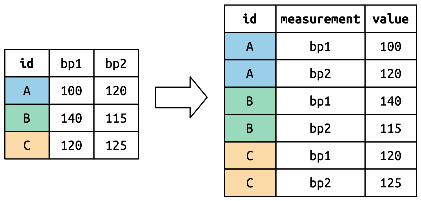
Values in columns that are already variables (here, id) need to be repeated for each pivoted column.

Understanding `pivot_longer()`

df |>
  pivot_longer(
    cols = c(bp1, bp2),  # which columns need to be pivoted
    names_to = "measurement",  # name of the column that the pivoted column names go
    values_to = "value"  # name of the column that the pivoted cell values go
  )

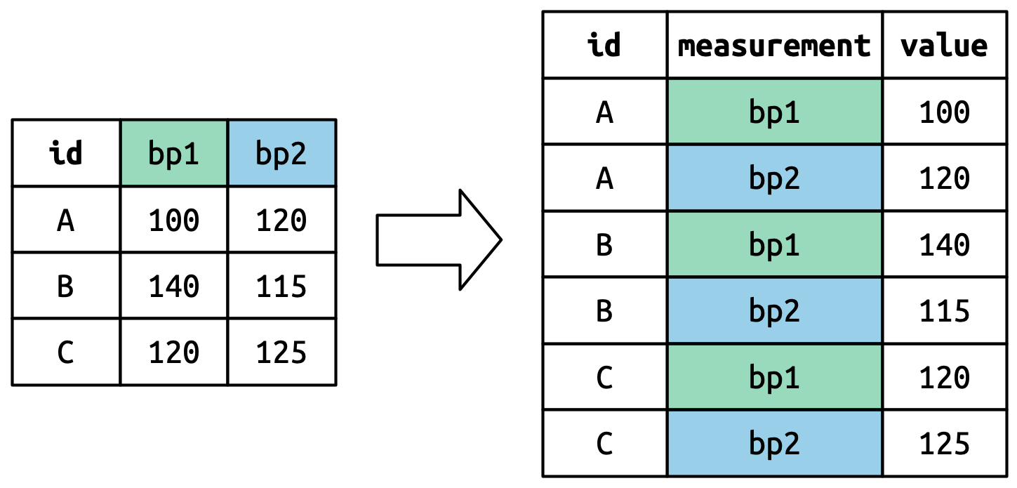
Pivoted column names bp1,bp2 become values in new column "measurement"; values repeated for each row in df.

Understanding `pivot_longer()`

df |>
  pivot_longer(
    cols = c(bp1, bp2),  # which columns need to be pivoted
    names_to = "measurement",  # name of the column that the pivoted column names go
    values_to = "value"  # name of the column that the pivoted cell values go
  )

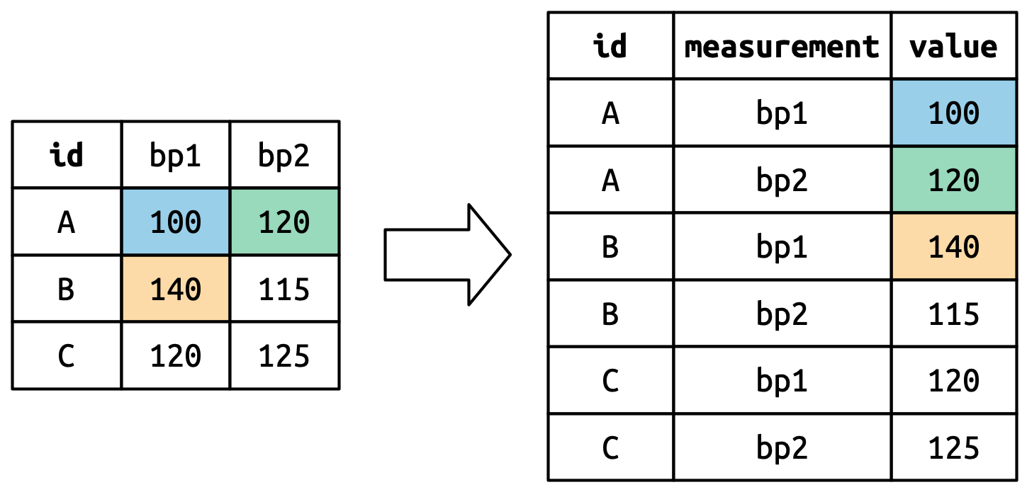
Cell values are values in a new variable, with name values_to, unwound row by row.

Widening data

We’ll now use pivot_wider() to widen data which is (too) long.

cms_patient_experience <- tidyr::cms_patient_experience |> 
   select(-measure_title)
cms_patient_experience

# A tibble: 500 × 4
   org_pac_id org_nm                               measure_cd   prf_rate
   <chr>      <chr>                                <chr>           <dbl>
 1 0446157747 USC CARE MEDICAL GROUP INC           CAHPS_GRP_1        63
 2 0446157747 USC CARE MEDICAL GROUP INC           CAHPS_GRP_2        87
 3 0446157747 USC CARE MEDICAL GROUP INC           CAHPS_GRP_3        86
 4 0446157747 USC CARE MEDICAL GROUP INC           CAHPS_GRP_5        57
 5 0446157747 USC CARE MEDICAL GROUP INC           CAHPS_GRP_8        85
 6 0446157747 USC CARE MEDICAL GROUP INC           CAHPS_GRP_12       24
 7 0446162697 ASSOCIATION OF UNIVERSITY PHYSICIANS CAHPS_GRP_1        59
...

The basic unit studied is an organization, but it’s spread across six rows for different measurements.

Widening data

cms_patient_experience |>
  pivot_wider(
    id_cols = starts_with("org"), # org_pac_id and org_nm are identifiers
    names_from = measure_cd,
    values_from = prf_rate
  )

# A tibble: 95 × 8
   org_pac_id org_nm CAHPS_GRP_1 CAHPS_GRP_2 CAHPS_GRP_3 CAHPS_GRP_5 CAHPS_GRP_8
   <chr>      <chr>        <dbl>       <dbl>       <dbl>       <dbl>       <dbl>
 1 0446157747 USC C…          63          87          86          57          85
 2 0446162697 ASSOC…          59          85          83          63          88
 3 0547164295 BEAVE…          49          NA          75          44          73
 4 0749333730 CAPE …          67          84          85          65          82
 5 0840104360 ALLIA…          66          87          87          64          87
 6 0840109864 REX H…          73          87          84          67          91
...

If you don’t supply id_cols, R assumes that all columns EXCEPT for names_from and values_from are id_cols.

Understanding `pivot_wider()`

Dataset where two patients (A, B), with between 2 and 3 BP measurements.

df

# A tibble: 5 × 3
  id    measurement value
  <chr> <chr>       <dbl>
1 A     bp1           100
2 B     bp1           140
3 B     bp2           115
4 A     bp2           120
5 A     bp3           105

df |>
  pivot_wider(
    names_from = measurement,
    values_from = value
  )

# A tibble: 2 × 4
  id      bp1   bp2   bp3
  <chr> <dbl> <dbl> <dbl>
1 A       100   120   105
2 B       140   115    NA

There is no measurement for bp3 for B, so R puts in NA.
id_cols is empty, so R assumes that all columns EXCEPT for names_from and values_from are id_cols.

Going from long to wide and back again

df

# A tibble: 5 × 3
  id    measurement value
  <chr> <chr>       <dbl>
1 A     bp1           100
2 B     bp1           140
3 B     bp2           115
4 A     bp2           120
5 A     bp3           105

(wide_df <- df |>
  pivot_wider(
    names_from = measurement,
    values_from = value
  ) )

# A tibble: 2 × 4
  id      bp1   bp2   bp3
  <chr> <dbl> <dbl> <dbl>
1 A       100   120   105
2 B       140   115    NA

(long_df <- wide_df |>
    pivot_longer(
      cols = c(bp1, bp2, bp3),
      names_to = "measurement",
      values_to = "value"))

# A tibble: 6 × 3
  id    measurement value
  <chr> <chr>       <dbl>
1 A     bp1           100
2 A     bp2           120
3 A     bp3           105
4 B     bp1           140
5 B     bp2           115
6 B     bp3            NA

We now have an additional row to account for the NA.

Tidy check

df

# A tibble: 8 × 4
  City  Date       Measurement Value
  <chr> <chr>      <chr>       <dbl>
1 CityA 2024-01-01 Temperature    20
2 CityA 2024-01-01 Humidity       80
3 CityA 2024-01-02 Temperature    22
4 CityA 2024-01-02 Humidity       82
5 CityB 2024-01-01 Temperature    18
6 CityB 2024-01-01 Humidity       85
7 CityB 2024-01-02 Temperature    19
8 CityB 2024-01-02 Humidity       88

Not tidy, since each variable is not a column, e.g. temperature/humidity.
“Tidyness” can be a bit ambiguous, but if a column has different units (e.g., degrees vs. % humidity), likely not tidy.
Q: How do we make the table wider?

Tidy check

df |>
  pivot_wider(
    names_from = Measurement,
    values_from = Value
  )

# A tibble: 4 × 4
  City  Date       Temperature Humidity
  <chr> <chr>            <dbl>    <dbl>
1 CityA 2024-01-01          20       80
2 CityA 2024-01-02          22       82
3 CityB 2024-01-01          18       85
4 CityB 2024-01-02          19       88

Tidy check

scores

# A tibble: 3 × 3
  Student  Math  Chem
  <chr>   <dbl> <dbl>
1 Alice      85    90
2 Bob        92    78
3 Charlie    88    95

Make scores longer by having a column called Subject with values "Math" and "Chem".

Q: Is the following code correct?

scores |>
  pivot_longer(
    cols = c(Math, Chem),
    names_to = Subject,
    values_to = Score
  )

No: scores tries to refer to Subject and Score which are not columns.

scores |>
  pivot_longer(
    cols = c(Math, Chem),
    names_to = "Subject",
    values_to = "Score"
  )

# A tibble: 6 × 3
  Student Subject Score
  <chr>   <chr>   <dbl>
1 Alice   Math       85
2 Alice   Chem       90
3 Bob     Math       92
4 Bob     Chem       78
5 Charlie Math       88
6 Charlie Chem       95

Complex calculations

Q: For each origin airport, compute the average flight time, in hours, for flights over 500 miles long.

colnames(flights)  # hint: use origin, air_time, distance

 [1] "year"           "month"          "day"            "dep_time"      
 [5] "sched_dep_time" "dep_delay"      "arr_time"       "sched_arr_time"
 [9] "arr_delay"      "carrier"        "flight"         "tailnum"       
[13] "origin"         "dest"           "air_time"       "distance"      
[17] "hour"           "minute"         "time_hour"

Complex calculations

Q: For each origin airport, compute the average flight time, in hours, for flights over 500 miles long.

flights |>
  mutate(air_time_hrs = air_time / 60) |>
  filter(distance > 500) |>
  group_by(origin) |>
  summarize(avg_flight_time_hrs = mean(air_time_hrs, na.rm=TRUE))

# A tibble: 3 × 2
  origin avg_flight_time_hrs
  <chr>                <dbl>
1 EWR                   2.99
2 JFK                   3.76
3 LGA                   2.27

Complex calculations

Q: For each origin airport, compute the average flight time, in hours, for flights over 500 miles long vs. less than or equal to 500 miles long.

colnames(flights)  # hint: use origin, air_time, distance

 [1] "year"           "month"          "day"            "dep_time"      
 [5] "sched_dep_time" "dep_delay"      "arr_time"       "sched_arr_time"
 [9] "arr_delay"      "carrier"        "flight"         "tailnum"       
[13] "origin"         "dest"           "air_time"       "distance"      
[17] "hour"           "minute"         "time_hour"

Complex calculations

Q: For each origin airport, compute the average flight time, in hours, for flights over 500 miles long vs. less than or equal to 500 miles long.

We will need to group_by() two variables:

origin airport
whether flight is $> 500$ or $\leq 500$ miles. (We need to create this variable.)

flights |>
  select(origin, air_time, distance) |>  # for visual clarity, not actually needed
  mutate(air_time_hrs = air_time / 60,
         distance_greater_500mi = distance > 500)

# A tibble: 336,776 × 5
   origin air_time distance air_time_hrs distance_greater_500mi
   <chr>     <dbl>    <dbl>        <dbl> <lgl>                 
 1 EWR         227     1400        3.78  TRUE                  
 2 LGA         227     1416        3.78  TRUE                  
 3 JFK         160     1089        2.67  TRUE                  
 4 JFK         183     1576        3.05  TRUE                  
...

Complex calculations

Q: For each origin airport, compute the average flight time, in hours, for flights over 500 miles long vs. less than or equal to 500 miles long.

flights |>
  mutate(air_time_hrs = air_time / 60,
         distance_greater_500mi = distance > 500) |>
  group_by(origin, distance_greater_500mi) |>
  summarize(avg_flight_time_hrs = mean(air_time_hrs, na.rm=TRUE))

# A tibble: 6 × 3
# Groups:   origin [3]
  origin distance_greater_500mi avg_flight_time_hrs
  <chr>  <lgl>                                <dbl>
1 EWR    FALSE                                0.900
2 EWR    TRUE                                 2.99 
3 JFK    FALSE                                0.849
4 JFK    TRUE                                 3.76 
5 LGA    FALSE                                0.916
6 LGA    TRUE                                 2.27

Operating on logical vectors

Intro

For logical vectors, every element takes one of 3 values: TRUE, FALSE, NA

We’ll investigate how to manipulate and transform data to get logicals, and how to use logicals.

library(tidyverse)
library(nycflights13)
flights

# A tibble: 336,776 × 19
    year month   day dep_time sched_dep_time dep_delay arr_time sched_arr_time
   <int> <int> <int>    <int>          <int>     <dbl>    <int>          <int>
 1  2013     1     1      517            515         2      830            819
 2  2013     1     1      533            529         4      850            830
 3  2013     1     1      542            540         2      923            850
 4  2013     1     1      544            545        -1     1004           1022
...

Three basic logical operators that we will use over and over:

AND (denoted & in R): operation between two logicals
OR (denoted | in R): operation between two logicals
NOT (denoted ! in R): operation on a single logical.

Truth table for AND:

A	B	A `&` B
`TRUE`	`TRUE`	`TRUE`
`TRUE`	`FALSE`	`FALSE`
`FALSE`	`TRUE`	`FALSE`
`FALSE`	`FALSE`	`FALSE`

Truth table for OR:

A	B	A `\|` B
`TRUE`	`TRUE`	`TRUE`
`TRUE`	`FALSE`	`TRUE`
`FALSE`	`TRUE`	`TRUE`
`FALSE`	`FALSE`	`FALSE`

Truth table for NOT:

A	`!` A
`TRUE`	`FALSE`
`FALSE`	`TRUE`

Can combine AND/OR with NOT to cover any binary Boolean operation

Comparisons

Common way to create a logical vector: numeric comparison with <, !=, etc.

We have implicitly been using this when doing filtering.

flights$dep_time > 600

    [1] FALSE FALSE FALSE FALSE FALSE FALSE FALSE FALSE FALSE FALSE FALSE FALSE
   [13] FALSE FALSE FALSE FALSE FALSE FALSE FALSE  TRUE  TRUE  TRUE  TRUE  TRUE
...

Using a comparator between two vectors of logicals returns pairwise comparisons.

x <- c(TRUE, FALSE, TRUE)
y <- c(FALSE, FALSE, TRUE)
(x & y) # x AND y

[1] FALSE FALSE  TRUE

(x | y) # x OR y

[1]  TRUE FALSE  TRUE

Comparisons

So when we use multiple comparisons in filter(), we are building a new vector of logicals.

We only keep those rows where the vector is TRUE.

flights |>
  filter(dep_time > 600 & dep_time < 2000 & abs(arr_delay) < 20)

# A tibble: 172,286 × 19
    year month   day dep_time sched_dep_time dep_delay arr_time sched_arr_time
   <int> <int> <int>    <int>          <int>     <dbl>    <int>          <int>
 1  2013     1     1      601            600         1      844            850
 2  2013     1     1      602            610        -8      812            820
 3  2013     1     1      602            605        -3      821            805
...

Comparisons

filter() and mutate() can be used in conjunction

flights |>
  mutate(
    daytime = dep_time > 600 & dep_time < 2000,
    approx_ontime = abs(arr_delay) < 20,
  ) |>
  filter(daytime & approx_ontime)

# A tibble: 172,286 × 21
    year month   day dep_time sched_dep_time dep_delay arr_time sched_arr_time
   <int> <int> <int>    <int>          <int>     <dbl>    <int>          <int>
 1  2013     1     1      601            600         1      844            850
 2  2013     1     1      602            610        -8      812            820
 3  2013     1     1      602            605        -3      821            805
...

Floating point comparisons

Testing equality with == for floating points can cause problems. Numbers are represented with finite “precision”, i.e. only up to 2^{-32} or 2^{-64}.

x <- c( (1/49) * 49, sqrt(2)^2)
x == c(1,2)

[1] FALSE FALSE

What’s going on? Let’s look at more precise representation in R.

print(x, digits=10)

[1] 1 2

print(x, digits=20)

[1] 0.99999999999999988898 2.00000000000000044409

dplyr::near() helps with this, ignores small differences

near(x, c(1,2))

[1] TRUE TRUE

all.equal(x, c(1,2))  # returns single value

[1] TRUE

Missing values

Almost any operation involving an NA returns NA.

(NA > 5)

[1] NA

(10 == NA)

[1] NA

What about NA==NA?

NA==NA

[1] NA

Why? Think of this example

# Suppose we don't know Ant's age
age_ant <- NA

# And we also don't know Bug's age
age_bug <- NA

# Then we shouldn't know whether Ant and
# Bug are the same age
age_ant == age_bug

[1] NA

Missing values

A useful function for dealing with NA: is.na()

is.na(x) works with any type of vector and returns TRUE for missing values and FALSE for everything else:

is.na(c(TRUE, NA, FALSE))

[1] FALSE  TRUE FALSE

is.na(c(1, NA, 3))

[1] FALSE  TRUE FALSE

is.na(c("a", NA, "b"))

[1] FALSE  TRUE FALSE

Missing values

Since is.na() returns logicals, can be used in filter():

flights |>
  filter(is.na(dep_time))

# A tibble: 8,255 × 19
    year month   day dep_time sched_dep_time dep_delay arr_time sched_arr_time
   <int> <int> <int>    <int>          <int>     <dbl>    <int>          <int>
 1  2013     1     1       NA           1630        NA       NA           1815
 2  2013     1     1       NA           1935        NA       NA           2240
...

Missing values

Can use to help identify where NA come from. e.g., why are there air_time NAs?

Let’s examine how dep_time, dep_delay, and sched_dep_time are related.

flights |> 
  mutate(missing_dep_time = is.na(dep_time),
         missing_dep_delay = is.na(dep_delay),
         missing_sched_dep_time = is.na(sched_dep_time)) |> 
  count(missing_dep_time, missing_dep_delay, missing_sched_dep_time)

# A tibble: 2 × 4
  missing_dep_time missing_dep_delay missing_sched_dep_time      n
  <lgl>            <lgl>             <lgl>                   <int>
1 FALSE            FALSE             FALSE                  328521
2 TRUE             TRUE              FALSE                    8255

The only instances where dep_delay is missing have dep_time missing.

Missing values

Is it the case that dep_delay = dep_time - sched_dep_time?

flights |> 
  mutate(dep_delay_manual = dep_time - sched_dep_time,
         manual_matches_given = near(dep_delay_manual, dep_delay)) |>
  count(manual_matches_given)

# A tibble: 3 × 2
  manual_matches_given      n
  <lgl>                 <int>
1 FALSE                 99777
2 TRUE                 228744
3 NA                     8255

Quite weird, since we are getting a lot right but also getting a lot wrong.

Missing values

Let’s inspect further. What do the mismatched observations look like?

flights |> 
  mutate(manual_delay = dep_time - sched_dep_time,
         manual_matches_given = near(manual_delay, dep_delay)) |>
  filter(!manual_matches_given) |>
  select(time_hour, flight, dep_time, sched_dep_time, dep_delay, manual_delay)

# A tibble: 99,777 × 6
   time_hour           flight dep_time sched_dep_time dep_delay manual_delay
   <dttm>               <int>    <int>          <int>     <dbl>        <int>
 1 2013-01-01 06:00:00    461      554            600        -6          -46
 2 2013-01-01 06:00:00    507      555            600        -5          -45
 3 2013-01-01 06:00:00   5708      557            600        -3          -43
...

Problem: R is treating dep_time and sched_dep_time as integers, not time!

5:54 is only 6 minutes away from 6:00, rather than 46.
We might discuss later (after midterm 2) how to properly treat dates and times.

Missing values in Boolean algebra

Logical and missing values interact in logical, but maybe counterintuitive ways.

Think of NA as “unknown” logical value.

tibble(x = c(TRUE, FALSE, NA)) |>  
  mutate(
    and_NA = x & NA,
    or_NA = x | NA
  )

# A tibble: 3 × 3
  x     and_NA or_NA
  <lgl> <lgl>  <lgl>
1 TRUE  NA     TRUE 
2 FALSE FALSE  NA   
3 NA    NA     NA

Does not depend on value of NA:

NA OR TRUE will return TRUE.
NA AND FALSE will return FALSE.

Depends on value of NA:

NA AND TRUE will return NA.
NA OR FALSE will return NA.

Consider finding all flights departing in November or December.

flights |>  # results in correct calculation
  filter(month == 11 | month == 12)

# A tibble: 55,403 × 19
    year month   day dep_time sched_dep_time dep_delay arr_time sched_arr_time
   <int> <int> <int>    <int>          <int>     <dbl>    <int>          <int>
 1  2013    11     1        5           2359         6      352            345
 2  2013    11     1       35           2250       105      123           2356
...

flights |>  # results in incorrect calculation. (we get all rows back)
  filter(month == 11 | 12)

# A tibble: 336,776 × 19
    year month   day dep_time sched_dep_time dep_delay arr_time sched_arr_time
   <int> <int> <int>    <int>          <int>     <dbl>    <int>          <int>
 1  2013     1     1      517            515         2      830            819
 2  2013     1     1      533            529         4      850            830
...

`%in%`

Instead of worrying about | and == in order, just use %in%.

1:10 %in% c(1, 5, 10)

 [1]  TRUE FALSE FALSE FALSE  TRUE FALSE FALSE FALSE FALSE  TRUE

So to find all flights from November and December:

flights |>
  filter(month %in% c(11, 12))

%in% obeys different rules for NA vs. ==, since NA %in% NA is TRUE:

(c(1,2,NA) == NA)

[1] NA NA NA

(c(1,2,NA) %in% NA)

[1] FALSE FALSE  TRUE

Logical summaries

Two main functions for logical summaries:

any(x) returns TRUE if any value in x is TRUE
all(x) returns TRUE only if all values in x are TRUE

For instance, was there a day where every flight was delayed on departure by less than an hour? Or a day where there were any flights delayed on arrival by $\leq 5$ hours?

flights |>
  group_by(year, month, day) |>
  summarize(
    all_delayed = all(dep_delay <= 60, na.rm=TRUE),
    any_long_delay = any(arr_delay >= 300, na.rm=TRUE)
  )

# A tibble: 365 × 5
# Groups:   year, month [12]
    year month   day all_delayed any_long_delay
   <int> <int> <int> <lgl>       <lgl>         
 1  2013     1     1 FALSE       TRUE          
 2  2013     1     2 FALSE       TRUE          
 3  2013     1     3 FALSE       FALSE         
 4  2013     1     4 FALSE       FALSE         
...

Logical summaries

When coerced into a numeric, TRUE coerces to 1 and FALSE coerces to 0
Useful if you want to find proportions that are TRUE/FALSE, e.g. mean(), sum()

Logical summaries

Example: proportion of flights delayed > 1 hour on departure, and number of flights delayed on arrival by > 5 hours:

flights |> 
  group_by(year, month, day) |>
  summarise(
    prop_delayed_1hour = mean(dep_delay > 60, na.rm=TRUE),
    num_long_delay = sum(arr_delay > 300, na.rm=TRUE)
  )

# A tibble: 365 × 5
# Groups:   year, month [12]
    year month   day prop_delayed_1hour num_long_delay
   <int> <int> <int>              <dbl>          <int>
 1  2013     1     1             0.0609              3
 2  2013     1     2             0.0856              3
 3  2013     1     3             0.0586              0
...

Note output: # Groups: year, month [12]

Logical summaries

Example: proportion of flights delayed > 1 hour on departure, and number of flights delayed on arrival by > 5 hours:

flights |> 
  group_by(year, month, day) |>
  summarise(
    prop_delayed_1hour = mean(dep_delay > 60, na.rm=TRUE),
    num_long_delay = sum(arr_delay > 300, na.rm=TRUE),
    .groups = 'drop'
  )

# A tibble: 365 × 5
    year month   day prop_delayed_1hour num_long_delay
   <int> <int> <int>              <dbl>          <int>
 1  2013     1     1             0.0609              3
 2  2013     1     2             0.0856              3
 3  2013     1     3             0.0586              0
...

Conditional transformations: `if_else()`

if_else(CONDITION, TRUE_VAL, FALSE_VAL, MISSING_VAL) is useful when we want to return some value when condition is TRUE and return another value when condition is FALSE.

x <- c(-2, -1, 1, 2, NA)
if_else(x > 0, "yay", "boo")

[1] "boo" "boo" "yay" "yay" NA

The fourth argument of if_else() specifies what to fill NA’s with:

if_else(x > 0, "yay", "boo", "idk how i feel about x yet")

[1] "boo"                        "boo"                       
[3] "yay"                        "yay"                       
[5] "idk how i feel about x yet"

We can also use vectors as an argument.

if_else(x < 0, -x, x)

[1]  2  1  1  2 NA

Conditional transformations: `if_else()`

We can use general vectors inside of if_else():

x1 <- c(NA, 1, 2, NA)
y1 <- c(3, NA, 4, 6)
if_else(is.na(x1), y1, x1)

[1] 3 1 2 6

Conditional transformations: `case_when()`

If you have many different conditions for which you want to specify values, e.g.

If number is between a and b then do…
If number is between b and c then do…
If number is between c and d then do…

You can use case_when().

Conditional transformations: `case_when()`

Inspired by SQL’s CASE statement. Has a very weird syntax:

condition ~ output
condition is a logical vector
when condition is TRUE, output is used.

Weird, but pretty readable:

x <- c(-3:3, NA)
case_when(
  x == 0   ~ "0",
  x < 0    ~ "-ve", 
  x > 0    ~ "+ve",
  is.na(x) ~ "???"
)

[1] "-ve" "-ve" "-ve" "0"   "+ve" "+ve" "+ve" "???"

Conditional transformations: `case_when()`

If no cases match, then returns NA:

x <- c(-2:2, NA)
case_when(
  x < 0 ~ "-ve",
  x > 0 ~ "+ve"
)

[1] "-ve" "-ve" NA    "+ve" "+ve" NA

If multiple conditions are satisfied, only the first is used – be careful!

case_when(
  x > 0 ~ "+ve",
  x > 2 ~ "big"
)

[1] NA    NA    NA    "+ve" "+ve" NA

The argument .default specifies return value if condition is satisfied, or if value is NA.

case_when(
  x < 0 ~ "-ve",
  x > 0 ~ "+ve",
  .default = "???"
)

[1] "-ve" "-ve" "???" "+ve" "+ve" "???"

`case_when()`: more complex example

Provide human-readable labels to flight delays.

flights |> 
  mutate(
    status = case_when(
      is.na(arr_delay)      ~ "cancelled",
      arr_delay < -30       ~ "very early",
      arr_delay < -15       ~ "early",
      abs(arr_delay) <= 15  ~ "on time",
      arr_delay < 60        ~ "late",
      arr_delay < Inf       ~ "very late",
    ),
    .keep = "used" # only returns those columns used in calculations
  )

# A tibble: 336,776 × 2
   arr_delay status 
       <dbl> <chr>  
 1        11 on time
 2        20 late   
...

We can refer to variables inside the dataframe inside case_when(), just as in most other tidyverse functions .
The first conditional that is true is what gets assigned.
So when arr_delay < -30, the remaining conditionals do not get checked.

Compatible types

Both if_else() and case_when() require the outputs to be of consistent types.

if_else(TRUE, "a", 1)
#> Error in `if_else()`:
#> ! Can't combine `true` <character> and `false` <double>.

case_when(
  x < -1 ~ TRUE,
  x > 0 ~ now()
)
#> Error in `case_when()`:
#> ! Can't combine `..1 (right)` <logical> and `..2 (right)` <datetime<local>>

Most types are incompatible in order to catch errors. Compatible types:

Numeric and logical (treats TRUE=1, FALSE=0)
Dates and “date-times” – we might discuss these types after midterm 2
NA is compatible with everything
Strings and factors are compatible

Example: labelling numbers as even or odd

Number is even $\Leftrightarrow$ number is divisible by two.
In R, operator %% (read “modulo”) does “modular arithmetic”:
a %% b returns the remainder when dividing a by b, e.g.
- 17 %% 12 = 5
- 34 %% 6 = 4
A number n is even if and only if n %% 2 == 0; otherwise, odd.
We can use if_else to label numbers between 0 and 20 as even or odd

x <- 0:20
if_else(x %% 2 == 0, 'even', 'odd')

 [1] "even" "odd"  "even" "odd"  "even" "odd"  "even" "odd"  "even" "odd" 
[11] "even" "odd"  "even" "odd"  "even" "odd"  "even" "odd"  "even" "odd" 
[21] "even"

Operating on numeric vectors

Parsing strings to get numbers

readr package in the tidyverse has two useful functions:

parse_double() – useful when you have numbers written as strings.
parse_number() – ignores all non-numeric text to parse strings.

parse_double(c("1.2", "5.6", "1e3"))

[1]    1.2    5.6 1000.0

parse_number(c("$1,234", "USD 53,256", "59%"))

[1]  1234 53256    59

Parsing strings to get numbers

What happens if use parse_double() with non-numeric-identifying strings?

x <- parse_double(c("qwerty", "6.5", "asdf"))
str(x)  # shows that x is a vector with informative attributes

 num [1:3] NA 6.5 NA
 - attr(*, "problems")= tibble [2 × 4] (S3: tbl_df/tbl/data.frame)
  ..$ row     : int [1:2] 1 3
  ..$ col     : int [1:2] NA NA
  ..$ expected: chr [1:2] "a double" "a double"
  ..$ actual  : chr [1:2] "qwerty" "asdf"

Can access this tibble by attributes(x)$problems

Arithmetic and “recycling rules”

We’ve created new rows before
- e.g. flights |> mutate(air_time_hr = air_time / 60).
- air_time has 336,776 elements while 60 has only one, so we divide every element of air_time by 60.
If you have two vectors of same length, operations are done element-wise:

x <- c(1, 2, 3, 4)
y <- c(2, 3, 4, 5)
x / y

[1] 0.5000000 0.6666667 0.7500000 0.8000000

Arithmetic and “recycling rules”

What happens if the number of elements is not 1 or the exact matching number?

R does what is called recycling, or repeating

It will create a new vector which repeats until reaches vector length.
Will throw warning if not an even multiple.

x <- c(-1, -2, -3, -4)
x * c(1,2)

[1] -1 -4 -3 -8

x * c(5, 6, 7)

Warning in x * c(5, 6, 7): longer object length is not a multiple of shorter
object length

[1]  -5 -12 -21 -20

Recycling rules

Rules apply for all logical comparison (==, <, etc) and arithmetic (+, ^, etc)

Be careful when doing logical comparisons / arithmetic using two vectors!

flights |> filter(month == c(1,2))

# A tibble: 25,977 × 19
    year month   day dep_time sched_dep_time dep_delay arr_time sched_arr_time
   <int> <int> <int>    <int>          <int>     <dbl>    <int>          <int>
 1  2013     1     1      517            515         2      830            819
 2  2013     1     1      542            540         2      923            850
 3  2013     1     1      554            600        -6      812            837
...

month == c(1,2) returns a logical vector where:
- TRUE if either the row number is odd and the month is 1, OR row number is even and month 2. Otherwise is FALSE.
Better to use month %in% c(1,2) here!

Parallel minimums and maximums

pmin() and pmax() return parallel min / max of 2 or more variables

df

# A tibble: 3 × 3
      x     y     z
  <dbl> <dbl> <dbl>
1     1     3     5
2     5     2     7
3     7    NA     1

df |> 
  mutate(min = pmin(x, y, z, na.rm=TRUE),
         max = pmax(x, y, z, na.rm=TRUE))

# A tibble: 3 × 5
      x     y     z   min   max
  <dbl> <dbl> <dbl> <dbl> <dbl>
1     1     3     5     1     5
2     5     2     7     2     7
3     7    NA     1     1     7

Parallel minimums and maximums

Different behavior than using min(), max(), which returns a single value:

df |>
  mutate(bad_min = min(x, y, z, na.rm=TRUE),
         bad_max = max(x, y, z, na.rm=TRUE))

# A tibble: 3 × 5
      x     y     z bad_min bad_max
  <dbl> <dbl> <dbl>   <dbl>   <dbl>
1     1     3     5       1       7
2     5     2     7       1       7
3     7    NA     1       1       7

Modular arithmetic

Recall from grade school: division by remainder.

%/%: integer division

1:10 %/% 3

 [1] 0 0 1 1 1 2 2 2 3 3

%%: the remainder after integer division.

1:10 %% 3

 [1] 1 2 0 1 2 0 1 2 0 1

Useful for time-related calculations, e.g. get hour and minute from sched_dep_time:

flights |> 
  mutate(hour = sched_dep_time %/% 100,
         minute = sched_dep_time %% 100,
         .keep = 'used')

# A tibble: 336,776 × 3
   sched_dep_time  hour minute
            <int> <dbl>  <dbl>
 1            515     5     15
 2            529     5     29
 3            540     5     40
 4            545     5     45
...

Modular arithmetic

We can then do things like calculate the percent of delayed flights per hour.

flights |> 
  mutate(hour = sched_dep_time %/% 100) |>
  group_by(hour) |>
  summarize(percent_cancelled = 100*mean(is.na(dep_time)),
            n = n())

# A tibble: 20 × 3
    hour percent_cancelled     n
   <dbl>             <dbl> <int>
 1     1           100         1
 2     5             0.461  1953
 3     6             1.64  25951
 4     7             1.27  22821
 5     8             1.62  27242
 6     9             1.61  20312
 7    10             1.74  16708
 8    11             1.85  16033
...

Rounding: `round()`

…to either nearest integer

round(pi)

[1] 3

…rounds (an integer + 0.5) to the nearest even integer

round(c(1.5, 2.5, 4.5, 5.5))

[1] 2 2 4 6

round(x, digits=n) rounds to n digits past the decimal place (if n>0)

round(123.456, digits=2)

[1] 123.46

round(123.456, digits=1)

[1] 123.5

What happens if n<0?

round(123.456, -1)

[1] 120

round(123.456, -2)

[1] 100

Rounding

Two similar functions: floor() and ceiling()

floor(x) rounds to greatest integer <= x
ceiling(x) rounds to least integer >= x.

floor(123.456)

[1] 123

ceiling(123.456)

[1] 124

Cumulative and rolling aggregates

R provides many functions for computing rolling (i.e., cumulative) aggregates

sums, products, minimums, etc.
cumsum(), cumprod(), cummin(), cummax(), dplyr::cummean()

x <- 9:1
cumsum(x)

[1]  9 17 24 30 35 39 42 44 45

cummean(x)

[1] 9.0 8.5 8.0 7.5 7.0 6.5 6.0 5.5 5.0

cumprod(x)

[1]      9     72    504   3024  15120  60480 181440 362880 362880

cummin(x)

[1] 9 8 7 6 5 4 3 2 1

Ranks: `dplyr::min_rank()`

Takes a vector of numbers and returns the rank of each element, with lowest = 1st.

min_rank(c(7,4,8,9))

[1] 2 1 3 4

Ties broken in obvious way: 1st, 2nd, 2nd, 4th if second and third element equal.

x <- c(62, 62, 64, NA, 20)
min_rank(x)

[1]  2  2  4 NA  1

To rank large values first, use desc(x):

min_rank(desc(x))

[1]  2  2  1 NA  4

There are many variants of min_rank() in dplyr:

row_number(), cume_dist(), percent_rank()
You can explore these on your own; min_rank() is enough in most cases.

Ranks: `dplyr::min_rank()`

Example: which 3 flight routes have the longest average delays?

flight route determined by origin and dest
negative arr_delay means the flight left early

flights |>
  filter(arr_delay > 0) |>
  group_by(origin, dest) |>
  summarize(avg_delay = mean(arr_delay, na.rm=TRUE),
            .groups = 'drop') |>
  mutate(rank = min_rank(desc(avg_delay))) |>
  filter(rank <= 3) |>
  arrange(by = rank)

# A tibble: 3 × 4
  origin dest  avg_delay  rank
  <chr>  <chr>     <dbl> <int>
1 LGA    TVC        72.7     1
2 EWR    TYS        72.6     2
3 LGA    OMA        65.0     3

Minimum, maximum, quantiles

Again, min(x) and max(x) return single smallest/largest vals within vector x.
quantile(vector, threshold) is a generalization of median:
- quantile(x, 0.25) returns value of x that is >= 25% of values within x
- quantile(x, 0.5) returns median
- quantile(x, 0.95) returns value of x that is >= 95% of values within x.
Compare to the mean, quantiles are less susceptible to extreme values
- Consider c(1, 2, 3, 2, 5, 2, 3, 1, 4, 2, 3, 1, 5, 2, 10000000)

Example: calculate the maximum delay and the 95th quantile of delays for flights per day.

flights |> 
  group_by(year, month, day) |>
  summarise(
    maxim = max(dep_delay, na.rm=TRUE),
    q95 = quantile(dep_delay, 0.95, na.rm=TRUE),
    .groups = 'drop'
  )

# A tibble: 365 × 5
    year month   day maxim   q95
   <int> <int> <int> <dbl> <dbl>
 1  2013     1     1   853  70.1
 2  2013     1     2   379  85  
 3  2013     1     3   291  68  
...

–>

s3: exploring data using tidyverse

Quick note

tidyverse

tidyverse approach to data manipulation

Reminder about packages

Load example dataset

Piping

Piping

Importing data

Introduction

read_csv(): can you spot the differences?

read_csv(): can you spot the differences?

Subsetting a data frame

Subset based on data values (rather than row/column indices)

The select() function

Helper functions for select()

The filter() function

The filter() function

Examples of filter()

Spot the error?

Spot the error?

Equivalent ways to filter on multiple conditions

Inspect a data frame

count()

count()

Summary statistics and missing data

summarise()

summarize()

group_by() and summarise()

group_by() and summarise()

mutate()

mutate()

mutate()

Reshaping a data frame

Tidy data

Tidy data

Tidying data

Lengthening data with pivot_longer()

Lengthening data with pivot_longer()

Lengthening data with pivot_longer()

Lengthening data with pivot_longer()

Understanding pivot_longer()

Understanding pivot_longer()

Understanding pivot_longer()

Understanding pivot_longer()

Widening data

Widening data

Understanding pivot_wider()

Going from long to wide and back again

Tidy check

Tidy check

Tidy check

Complex calculations

Complex calculations

Complex calculations

Complex calculations

Complex calculations

Complex calculations

Operating on logical vectors

Intro

Three basic logical operators that we will use over and over:

Comparisons

Comparisons

Comparisons

Floating point comparisons

Missing values

Missing values

Missing values

Missing values

Missing values

Missing values

Missing values in Boolean algebra

Consider finding all flights departing in November or December.

%in%

Logical summaries

Logical summaries

Logical summaries

Logical summaries

Conditional transformations: if_else()

Conditional transformations: if_else()

`tidyverse`

`tidyverse` approach to data manipulation

`read_csv()`: can you spot the differences?

`read_csv()`: can you spot the differences?

The `select()` function

Helper functions for `select()`

The `filter()` function

The `filter()` function

Examples of `filter()`

`count()`

`count()`

`summarise()`

`summarize()`

`group_by()` and `summarise()`

`group_by()` and `summarise()`

`mutate()`

`mutate()`

`mutate()`

Lengthening data with `pivot_longer()`

Lengthening data with `pivot_longer()`

Lengthening data with `pivot_longer()`

Lengthening data with `pivot_longer()`

Understanding `pivot_longer()`

Understanding `pivot_longer()`

Understanding `pivot_longer()`

Understanding `pivot_longer()`

Understanding `pivot_wider()`

`%in%`

Conditional transformations: `if_else()`

Conditional transformations: `if_else()`

Conditional transformations: `case_when()`

Conditional transformations: `case_when()`

Conditional transformations: `case_when()`

`case_when()`: more complex example

Rounding: `round()`

Ranks: `dplyr::min_rank()`

Ranks: `dplyr::min_rank()`